
Think of the curved lid of an elegant grand piano. The curve corresponds to the strings’ length, which corresponds to the perception of the pitch. This visual represents an important element of acoustics: Our perception of pitch is logarithmic. This means that there is a large frequency range involved in acoustics phenomena. In turn, when modeling acoustics problems, there is a large wavelength range to be meshed. But how?
Introduction to Free-Field FEM Wave Problems
A large frequency range needs to be computed, which means large wavelength ranges need to be resolved by the mesh. To efficiently mesh large frequency ranges, we can optimize the mesh element size by remeshing for a given frequency range when using finite element method (FEM) interfaces in the COMSOL Multiphysics® software.
The finite element method is implemented in most interfaces in COMSOL Multiphysics, including the Pressure Acoustics, Frequency Domain and the Pressure Acoustics, Transient interfaces. Other interfaces in the Acoustics Module are optimized for their intended purpose by implementing the boundary element method (BEM), ray tracing, or dG-FEM (time explicit). When using the Pressure Acoustics interface, FEM uses a mesh to discretize the geometry and solves the acoustic wave equation at these points. The full, continuous solution is interpolated from these points.
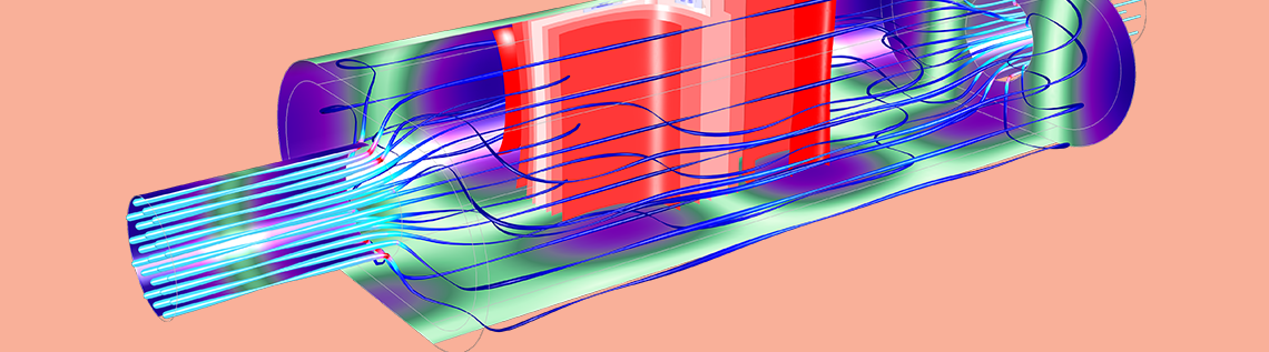
An automotive muffler with a porous lining, modeled using the pressure acoustics functionality in the COMSOL® software.
When meshing an FEM model, we need to get a good approximation of the geometry and include details of the physics. When using the Pressure Acoustics interface, we always need to resolve the acoustic waves. A good mesh resolves the geometry and the physics of the model, but a great mesh accurately solves the problem and also uses the smallest number of mesh elements possible. In this blog post, we will look at how to mesh free-field/open-ended problems with the fewest mesh points.
Mesh elements are comprised of nodes. For a linear mesh element, the nodes are located at the vertices. Second-order polynomial interpolation is the default shape function for wave equations in COMSOL Multiphysics. Second-order (or quadratic) elements have one additional node along the length of the element and resolve waves accurately. For free-field wave problems, we need to have about 10 or 12 nodes per wavelength to resolve the wave. Consequentially, for wave-based modeling with quadratic elements, we need 5 or 6 second-order elements per wavelength (hmax = \lambda_0/5). For short wavelengths (higher frequencies), the element size needs to be smaller than at lower frequencies.
Audio applications, which are concerned with human perception, have a frequency range of 20 Hz to 20 kHz. In air at room temperature, audio problems have a wavelength range from about 17 m to 17 mm. If we were to compute over the entire human auditory frequency range with one mesh, we would need to resolve for the wavelengths that correspond to 20 kHz. At the high-frequency end, this leads to a maximum element size, or spatial resolution, of (17 mm/5 =) 3.2 mm. Resolving the mesh for the highest frequency leads to an excessively dense mesh for the low-frequency predictions. At 20 Hz, the wavelength is 17 m and would have 5360 nodes per wavelength, far more than the 10 or 12 that is required. Each node corresponds to a memory allocation for the computer. While this dense mesh approach is great from an accuracy perspective, the excessively dense mesh takes up computational resources and consequentially takes longer time to compute.
Efficient Meshes in COMSOL Multiphysics®
Setup for Single-Octave Mesh
To avoid an inefficient meshing approach, we can split the problem into smaller frequency bands; initially, one octave, where the mesh for each frequency band is resolved according to its upper frequency limit. In this example, the center frequency, f_{C,n}, is referenced from f_0, the prescribed frequency,
f_{C,n} = 2^n \times f_0,
where n is the octave band number from the reference (positive n is higher-pitch octaves, negative n is lower-pitch octaves).
The upper and lower frequency band limits are defined from the center-band frequency
f_L = 2^{-\frac{1}{2}} \times f_{C,n} ,
f_U = 2^{\frac{1}{2}} \times f_{C,n}
Note that f_U is twice f_L (thus one octave higher).
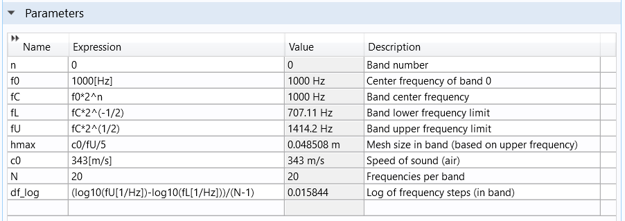
Defining the octaves in the model parameters.
We can use these parameters in the frequency-domain study using the range() function to define a logarithmic distribution of points within each band
10^{\textrm{range}(\log_{10}(f_L), df_\textrm{log}, \log_{10}(f_U) – df)},
The logarithmic frequency spacing, df_\textrm{log} = (\log_{10}(f_U)-\log_{10}(f_L))/(N-1), is set by the frequency range divided by the number of frequencies N.
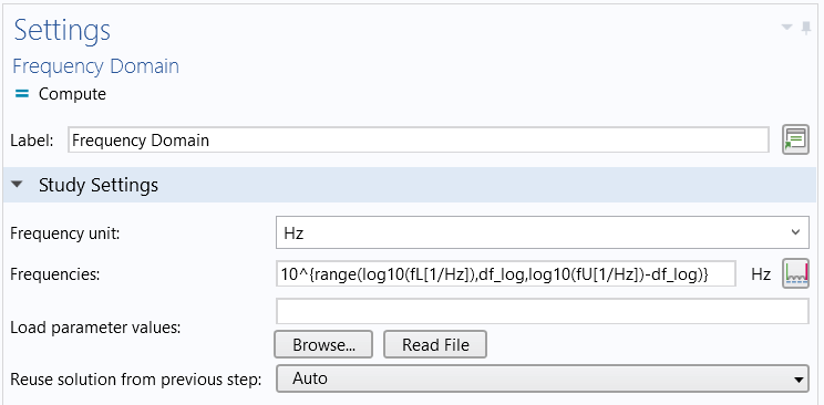
Setting the frequencies solved for in each octave band.
The maximum mesh element size (traditionally given the variable name hmax) is then taken from the higher limit of the given frequency band
hmax = 343[m/s]/f_U/5.
Note that if you do not know the speed of sound, you can use comp1.mat1.def.cs(23[degC]) to access the speed of sound for the first material (in a list), defined in Component 1 at 23°C. If you are using the built-in material Air, the speed of sound comes from the ideal gas law, so the fluid temperature is a required input.
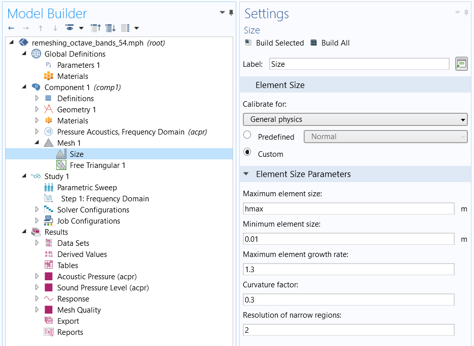
The custom mesh sequence with the parameter hmax applied to the Maximum element size.
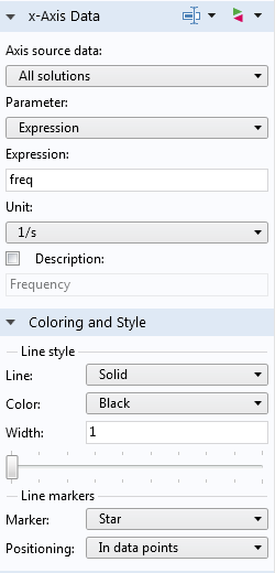
The Maximum element size is applied to the mesh on the Size node. The elements can be smaller than this constraint if smaller geometry details needs to be resolved, as shown in the figure below. The smallest element is controlled by the Minimum element size setting. The Curvature factor and Resolution of narrow regions settings are also important mesh settings.
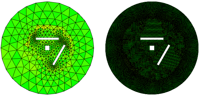
The mesh element quality shown on the top for two octave bands.
Setup for Multiple Octave Bands
If the COMSOL Multiphysics model is set up as described above, it would yield one octave’s worth of frequencies. However, we need up to 10 octaves for our audio investigations.
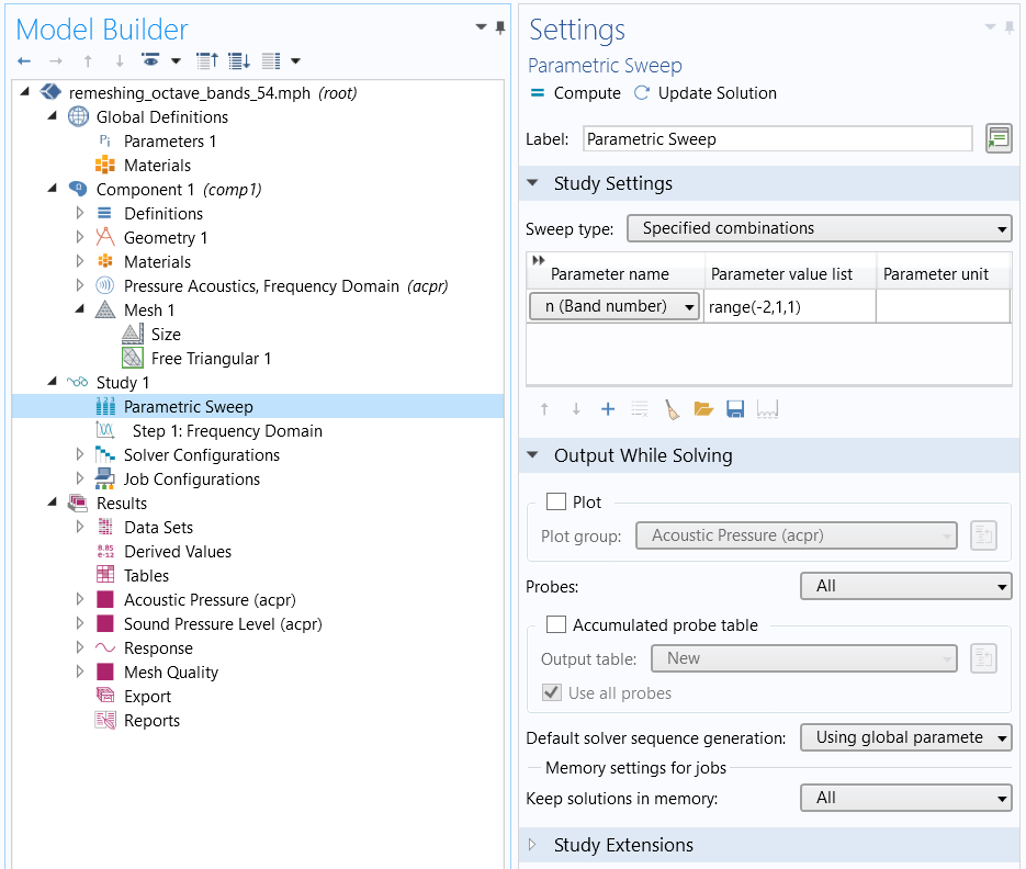
A parametric sweep over n, such that each value of n is an octave and the upper and lower frequency limits change accordingly.
To implement a parametric sweep in COMSOL Multiphysics, a Parametric Sweep study step is added to the study to change the frequency bands. The benefit of working with parameters is that all of the frequency band limits change automatically when the parameter sweep variable n changes. The parameter n is the natural choice for the parameter sweep because each value of n corresponds to a frequency band. Setting it up in this way means that the original frequency is now the reference frequency and must be chosen appropriately.
For the results shown below, the same frequencies were computed over the same range with the mesh for the highest frequency. The study that splits the mesh according to the octave band number took 32 s, whereas the single-mesh approach took 79 s. This shows a significant savings of time and computational resources.
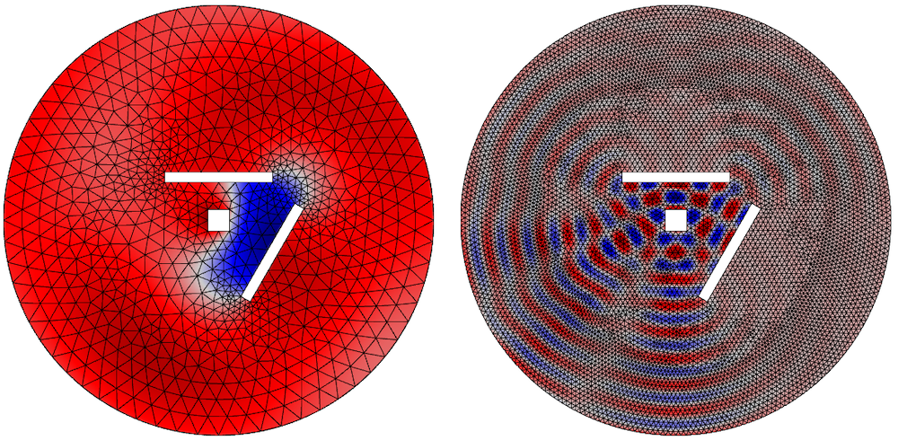
The instantaneous pressure is shown on the bottom for the different frequencies and meshes.
The Octave Band plot type is used to calculate the required response. Ensure that the line markers are placed in data points. Alternatively, to obtain a continuous line, change the x-Axis Data to Expression and enter freq, the variable for frequency.
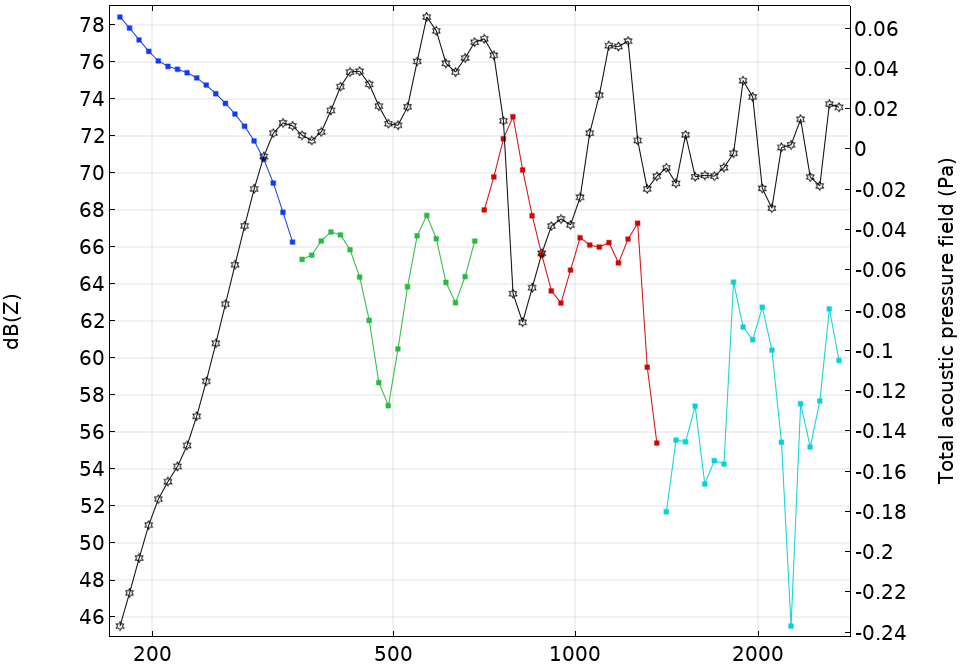
Plotting the continuous line.
Choose Point Graph and ensure that the plot settings are set up as shown above.
Setup for nth-Octaves Bands
The previous discussion sets up the problem in octave bands. However, you can use the general form of
f_{C,n} = 2^\frac{n}{b} \times f_0
f_L = 2^{-\frac{1}{2b}} \times f_{C,n} ,
f_U = 2^{\frac{1}{2b}} \times f_{C,n} ,
to allow fractions of octave bands. In the above setup, let b = 3 for third octave bands or 6 for sixth octave bands. The narrower the frequency band, the more times the meshing sequence runs, so there is a balance to be struck.
The parameters that set up the general meshing procedure in any octave band are located in the Remeshing in Frequency Bands model. It is easy to save the necessary parameters in a .txt file and load them when setting up a new model. This avoids having to enter them every time.
Discussion and Caveats of Meshing in Frequency Bands for Acoustics Simulations
The method presented in this blog post uses canonical geometry to clearly illustrate the process for optimizing the mesh. Consequentially, the meshing routine takes relatively little time. For realistic geometries, the meshing routine may take longer and the benefits may be less marked. In this instance, you should defeature or use virtual operations to reduce any physically irrelevant geometry.
For some problems, the temperature or density of the fluid may change significantly over the computational domain. If this occurs, the speed of sound will change and must be included in the model. The mesh must be dense enough to reflect this.
This discussion is not relevant to the Ray Tracing, Pressure Acoustics, Boundary Element, or Acoustic Diffusion interfaces. With care, the information in this blog post can be applied to free-field problems of the Aeroacoustics and Thermoviscous Acoustics interfaces or the dG-FEM-based Ultrasound interfaces. The convective effect of the flow alters the wavelength, and a sophisticated mesh should reflect this up- or downstream of a source. The Linearized Navier-Stokes and Linearized Euler interfaces have default linear interpolation, so 10 or 12 elements are required per wavelength. The Thermoviscous Acoustics interface is designed for resolving the acoustic boundary layer. The thickness of this layer is also frequency dependent, and a similar method to the one discussed here can be used for efficient meshing and resolution of the layer.
Finally, the discussion in this blog post explicitly assumes that the wavelength is known. This assumption is usually the case for free-field modeling, however for bounded, resonant problems, the total sound field is dependent on boundary condition values and the location of the boundaries. This means that the pressure amplitudes can have shapes with an analogous wavelength that could be significantly shorter than the free-field wavelength. To get an accurate solution, you must perform a mesh convergence study.
Conclusion
This blog post has demonstrated that remeshing in frequency bands can save a significant amount of time. In COMSOL Multiphysics, this is implemented by parameterizing the upper- and lower-frequency band limits. The approach demonstrated here is applicable for interfaces that implement FEM and have quadratic interpolation.
Next Steps
Try it yourself: Click the button below to access the MPH-file for the model discussed in this blog post.
Read More
Learn more about how to enhance your meshing processes on the COMSOL Blog:

Comments (3)
Roberto Magalotti
June 26, 2019The wavelength of a 20 kHz sound in air is 17 mm, not 17 cm. Since wavelength scales inversely with frequency, a mesh having 5 elements per wavelength at 20 kHz would have 5000 elements per wavelength at 20 Hz, not 500.
James Gaffney
June 27, 2019Thank you for pointing that out, Robert
Ahlam Altmimi
February 16, 2021I want to learn a validations of mesh method