

Vibration in rotating machinery is very sensitive to the geometric, structural, and inertial properties of the various rotating and stationary components interacting with each other. These properties include the location of the mounted components and their inertial properties, bearing characteristics, and shaft properties. To understand the effects of these parameters, start with a simple model and perform various analyses to correlate the rotor response within the same model. Let’s demonstrate this process with a simply supported beam rotor example.
2 Analysis Types for a Simply Supported Beam Rotor System
The rotor system in this example is a simple rotor with a uniform cross section throughout its length. It is supported at both ends by bearings and there are three mounted components called disks at different locations of the rotor.
You can model this rotor using the Beam Rotor interface in the COMSOL Multiphysics® software. The inertial properties and offset of the rotor components are modeled with the Disk node. The bearing support is modeled by an equivalent stiffness-based approach via the Journal Bearing node provided in the Beam Rotor interface.
For more information about the geometric properties and model setup, check out the references in the model documentation.
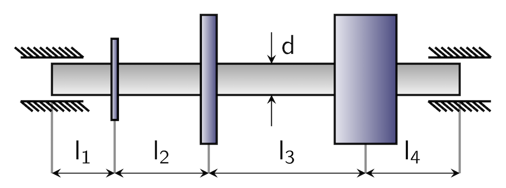
Geometry of the beam rotor example.
Two types of analyses are commonly used to study rotor vibration characteristics: eigenfrequency and time-domain analyses. As mentioned in a previous blog post, critical speeds of the rotor strongly depend on the rotor’s angular speed. Therefore, while performing the eigenfrequency analysis, you need to consider the variation in the rotor speed to get the correct critical speeds. A time-domain analysis is performed when you want to look at the system response under time-varying excitation.
Now, let’s look at what type of information each analysis provides as well as the steps involved to perform these analyses.
Eigenfrequency Analysis of a Rotor
Eigenfrequency analysis is used to determine the natural frequencies of a system. In a rotordynamics scenario, this analysis can be used in two different ways.
First, for the operating speed of a system that is not fixed, you can perform an eigenfrequency analysis of the system for the range of operating speeds and choose the one that is furthest from the critical speed of the system and meets other design considerations. If you cannot find a suitable operating speed for the current system, you might need to make certain design modifications in the system to get a stable operating speed that meets all of the requirements.
In the second type of analysis, the operating speed of the system is fixed. In such a case, you need to perform an eigenfrequency analysis at the given operating speed to check that any of the natural frequencies of the system are not close to the operating speed. If any of the natural frequencies fall closer to the operating speed, design modifications are a must.
The design modifications in the rotor system require an understanding of what kind of modifications will produce the desired effect and at what cost. This is where simulating simple systems to understand the effect of design modifications is very helpful. Simulation can provide guidelines for design modifications, thus reducing the number of iterations in the design process.
Consider the first case, in which the operating speed of the system is not fixed, to understand the analysis steps. In this case, you need to perform a parametric eigenfrequency analysis for the angular speed of the rotor. This requires two steps in the Study node: Parametric Sweep and Step 1: Eigenfrequency, shown below on the left. Settings for the Parametric Sweep node for a sweep over a parameter Ow representing the angular speed of the rotor are shown below in the center. This parameter is used as an input in the Rotor Speed section of the Beam Rotor node settings, shown below on the right.

Steps in the Study node (left), settings for the parametric sweep (middle), and rotor speed input (right).
After performing the analysis, you get a whirl plot of the rotor as the default, shown below. The whirl plot shows the whirling orbit and the deformed shape of the rotor for the given rpm and natural frequency combinations.
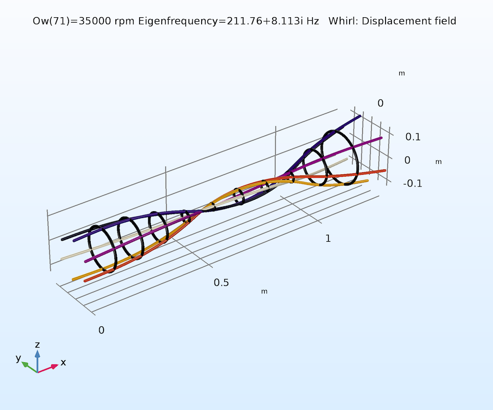
Whirl plot of the rotor.
The deformed shape of the rotor also gives you an idea of how strongly the natural frequency will depend on the angular speed of the rotor. If the disks move away from the rotation axis without significant tilting, then the split in the frequency in the backward whirl (opposite to the spin) and forward whirl (same direction as the spin) is not significant. Alternatively, if the disks do not move significantly far from the rotation axis and rather have significant tilting, then the split in the frequency of the backward and forward whirl is noticeable.
To understand this concept in depth, you can plot the variation of the natural frequency for different modes against the angular speed of the rotor, which is often called a Campbell diagram. The Campbell plot for the simply supported rotor example is shown below. You can see the strong divergence of the eigenfrequencies with rotor speed for certain modes; whereas for others, particularly the modes with low natural frequencies, the divergence is not significant. If you look at the mode shapes corresponding to these frequencies, they confirm the behavior previously discussed. Critical speeds of the rotor can be obtained from the Campbell plot by looking at the intersection of the natural frequency vs. angular speed curve with ω = Ω curve. These are the speeds near which a rotor should not be operated, unless sufficiently damped.
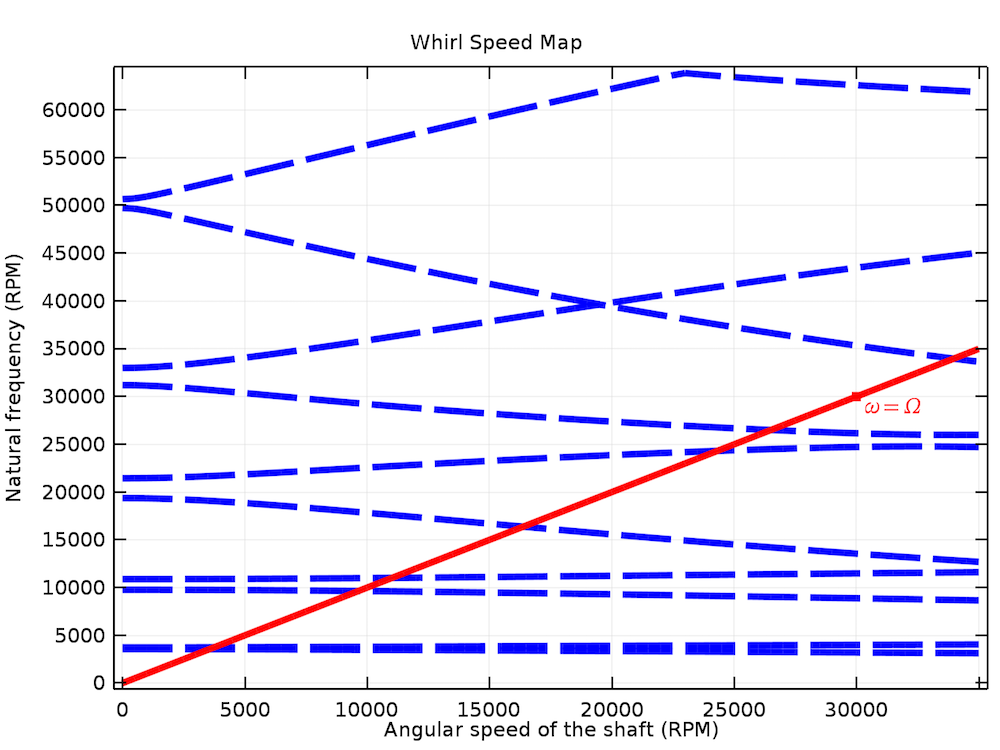
Campbell plot of the simply supported rotor system.
The damping in the respective modes can be accessed by plotting the logarithmic decrement with the angular speed of the rotor. The logarithmic decrement is defined as
where A(t) is a time-varying response and ω is the complex eigenfrequency of the system. T is the time period given by T = \frac{2\pi}{\Re(\omega)}.
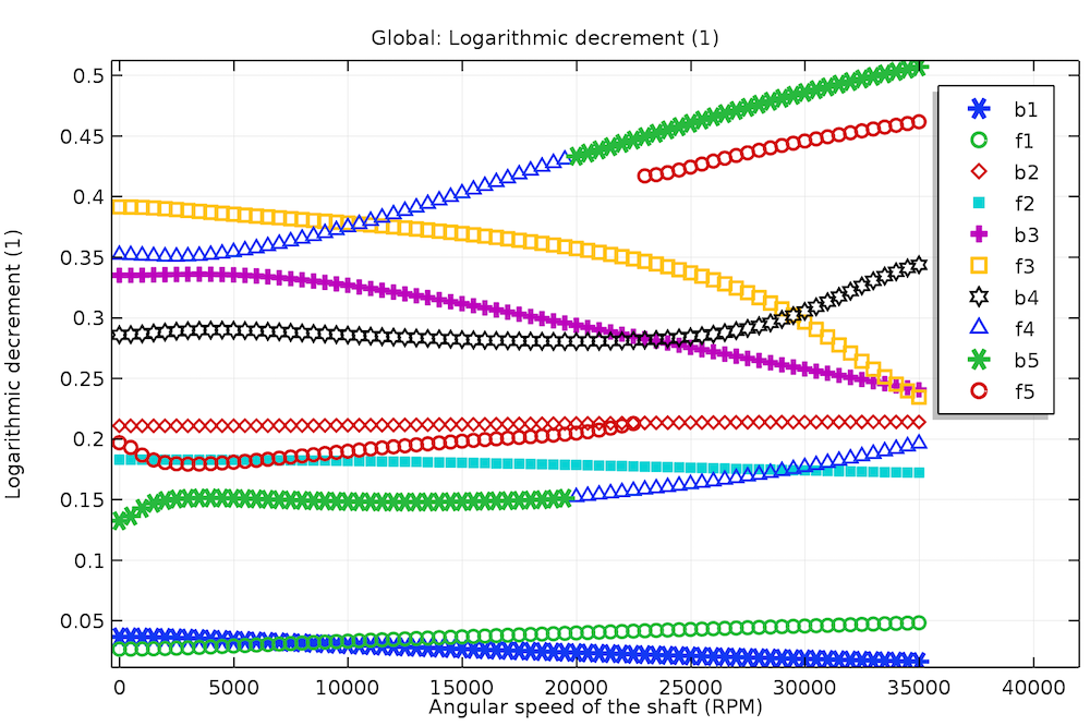
Logarithmic decrement for different bending modes in the simply supported rotor system.
In the plot above, you can see a logarithmic decrement variation for the different bending modes with the angular speed for the simply supported rotor. The notation ‘b’ and ‘f’ is used for the backward and forward whirl modes, respectively. A logarithmic decrement of zero means that the system is undamped, a negative value indicates an unstable system, and a positive value indicates a stable system.
You can also note the pattern change for some of the curves. The reason is that the modal data is arranged in increasing order of the natural frequency. But we know that the rotor’s natural frequencies decrease in the backward whirl modes and increase in the forward whirl modes. Due to this, there is crossover of the natural frequencies between the higher backward whirl and lower forward whirl modes beyond a certain angular speed. This upsets the initial order of the modes, resulting in switching of the patterns across the crossover points.
Time-Dependent Analysis of a Rotor
Eigenfrequency analysis gives the characteristics of the rotor system operating at steady state. However, before and after reaching the steady state, during the run-up and run-down, the angular speed of the rotor varies with time. In certain cases, the operating speed might be above the first few natural frequencies of the rotor. Therefore, during the run-up and run-down, the rotor will cross over the corresponding critical speeds. Also, there could be nonharmonic time-varying external excitation acting on the rotor. In such cases, the rotor response cannot be completely determined by an eigenfrequency or frequency-domain analysis. Rather, you need a time-dependent simulation to study the response of the system.
You can also perform a time-dependent analysis of the rotor at different angular speeds by performing a parametric sweep to see how the angular speed governs the response. An obvious extension of such an analysis is to evaluate the frequency spectrum of the time-dependent response of the rotor for all of the angular speeds and analyze what combinations of the angular speed and frequency result in a high amplitude response. A waterfall plot shows the response amplitude vs. angular speed and frequency and gives the distribution of the modal participation in the response at different speeds. Such an analysis can be set up using the three steps in the study node, as shown below.
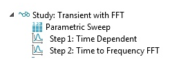
Steps for a waterfall plot analysis. The Parametric Sweep study step is used to sweep the angular speed, a Time Dependent study step is used to perform a time-dependent analysis corresponding to each angular speed in the parametric sweep, and a Time to Frequency FFT study step takes the fast Fourier transform of the time-dependent data to convert into the frequency spectrum.
In the eigenfrequency analysis, bearings are modeled using constant stiffness and damping coefficients. However, in reality, these coefficients are strongly dependent on the journal motion. To highlight the effect of the nonlinearity for the time-domain analysis, a plain journal bearing model is used instead of the constant bearing coefficients. A plain journal bearing model is based on the analytical solution of the Reynolds equation for a short bearing approximation. The system in this case is self-excited due to the eccentric mounting modeled as a disk. To simplify the system, only the second disk is considered with small eccentricity in the local y direction.
The waterfall plot of the z-component of the displacement is shown in the figure below. You can observe three peaks clearly in the spectrum. The third peak, which falls along the ω = Ω curve, corresponds to a 1X synchronous whirl. This is in response to the centrifugal force due to eccentricity changing its direction with the rotation of the shaft. Other peaks correspond to the orbiting of the rotor due to the complex rotor bearing interaction. The reason is that the forces from the pressure distribution around the journal in the bearing have a cross-coupling effect with the journal motion. In other words, the motion of the journal in one of the lateral directions induces a component of the force in the lateral direction perpendicular to it. The effect of this phenomenon is a net force acting on the rotor in the direction of the forward whirl. This causes the subsynchronous orbiting of the rotor.
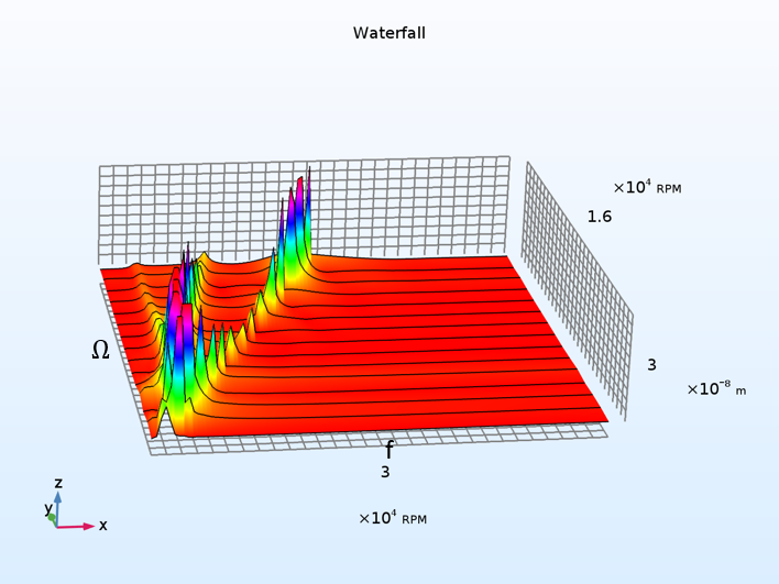
A waterfall plot shows the response amplitude vs. the angular speed and frequency of the rotor.
The orbit of the different locations along the length of the rotor at 30,000 rpm is shown below. The orbit curve changes its color from green to red with time. You can see that after the initial transient phase, the rotor undergoes a forward circular whirl in the steady state. Also, the second bending mode has the highest participation in the response.
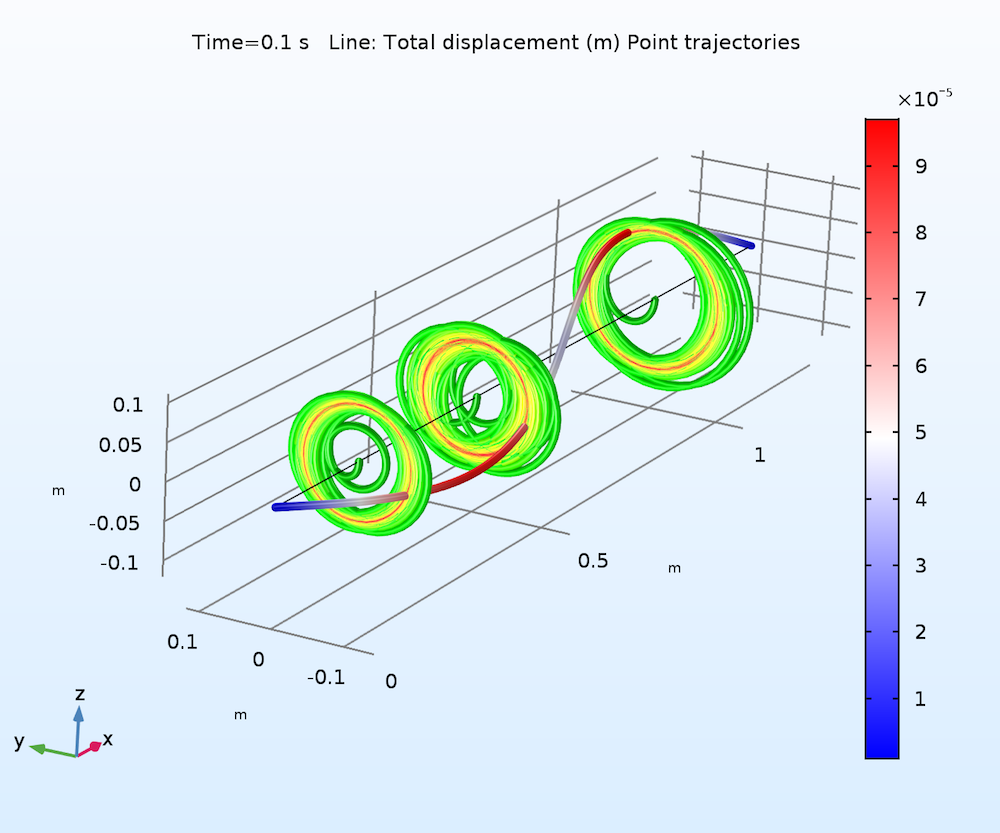
Orbit of the rotor at different locations. The plot changes from green to red with time.
The time variation of the z-direction displacement of a point on the rotor at 30,000 rpm is shown below. Apart from the high-frequency variation, there is also a low-frequency component that envelops the response, but gets damped out with time.
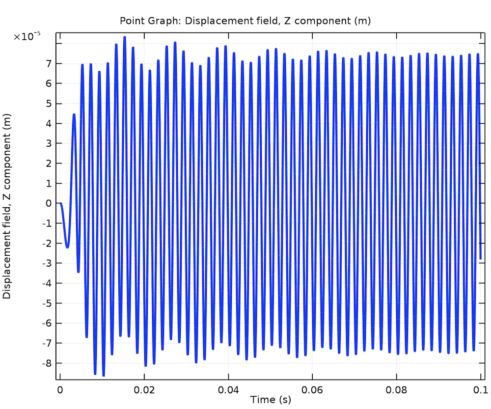
Time variation of the z-displacement.
With this tutorial model, we have demonstrated the approach to set up different analyses in a rotor system, as well as how to plot and analyze the simulation results. Ready to give this tutorial a try? Simply click on the button below to access the MPH-file via the Application Gallery or open it via the Application Library in the COMSOL® software.
Learn More About Analyzing Rotordynamics Applications
- Learn about the features included with the Rotordynamics Module
- See how to model a reciprocating engine to optimize its design

Comments (0)