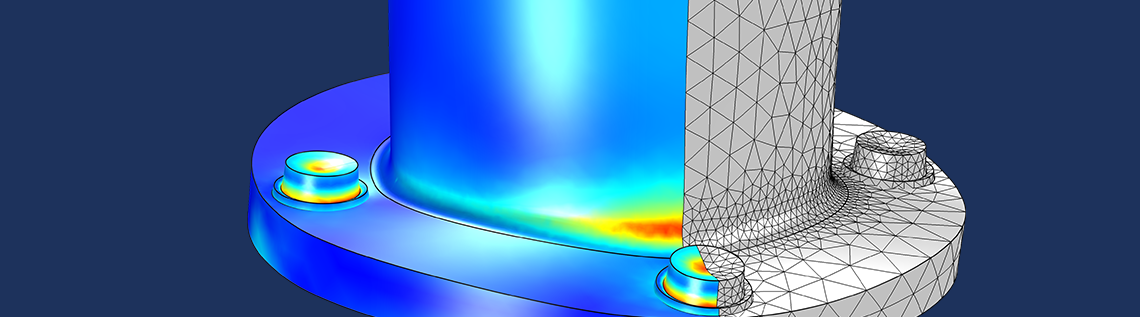

In some applications, it is necessary to approximate a general 3D stress state by a set of linearized stresses through a cross section of a thin structure. This is important for applications like the analysis of pressure vessels, fatigue analysis of welds, and determination of reinforcement requirements in concrete. In this blog post, we discuss why such an approach is useful as well as how to compute linearized stresses in the Structural Mechanics Module for COMSOL Multiphysics® version 5.3.
Defining Membrane and Bending Stresses
When performing a structural analysis with plate or shell elements, there is an underlying assumption that the variation of the in-plane stresses through the thickness is linear. In a local coordinate system, where z is oriented along the normal to the shell surface, it is thus possible to write
where d is the thickness. The indices i and j can be either x or y. In this decomposition, \sigma_{ij,m} is called the membrane stress and \sigma_{ij,b} (or \frac{2z}{d}\sigma_{ij,b}) is called the bending stress.
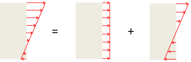
The decomposition of a linear stress distribution into a membrane stress and bending stress.
For the other stress components, shell theory implies that
and
Unless the shell is thick, the transverse shear stresses, σiz, are significantly smaller than the in-plane stresses.
Why Membrane Stresses Are More Dangerous
A membrane stress has the same value all through the section. If the material is assumed to be elastoplastic with no hardening, then all points reach the failure stress at the same time. The load that causes incipient plasticity is thus also the failure load.
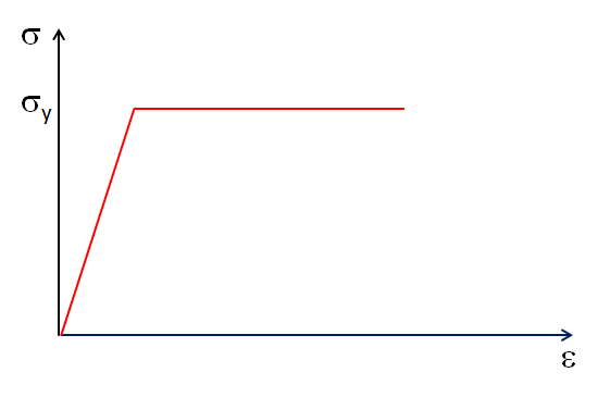
The stress-strain curve for an elastoplastic material with no hardening. The variable σy is the yield stress.
Now, consider pure bending with a uniaxial stress state, as in a beam. As long as the material is elastic, the stress distribution is linear through the section, with the value being zero at the midsurface. As the load increases, the stress in the outermost fibers reaches the yield limit. However, the rest of the section is still elastic. It is thus possible to further increase the load without a complete failure.
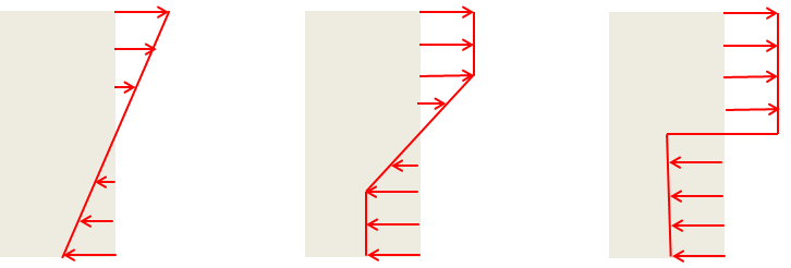
The stress distribution at incipient yielding (left), partly through yielding (middle), and collapse (right).
The bending moment at failure is 1.5 times the bending moment at initial yield. Thus, if the allowed stress only takes the maximum stress into account, the risk of collapse is larger for a membrane state than it is for a bending state.
If we consider a state of mixed bending and tension, it is possible to compute the combinations of moment, M, and axial force, N, which cause failure.
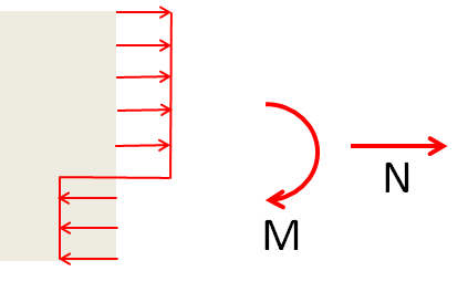
The stress state at collapse for combined tension and bending.
The membrane and bending stresses are, for an elastic case, related to the moment and axial force through
and
By writing the moment and axial force in terms of membrane and bending stresses, we arrive at the following interaction formula:
When the Detailed Stress Distribution Does Not Matter
In a full 3D case, the stress distribution differs significantly from linear in the vicinity of geometric discontinuities. This is where the concept of stress linearization becomes important. The sum of the membrane and bending stress provides a linear approximation to the true stress distribution, having the property that the resultant force and moment are preserved.
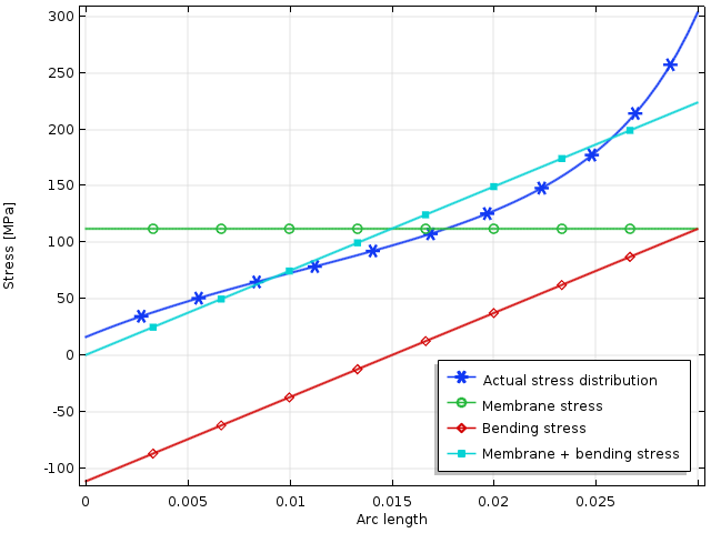
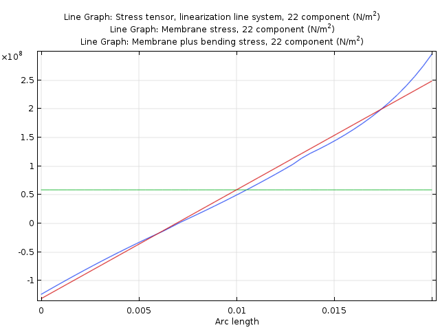
The linearization of a stress tensor component from a 3D solution.
In the graph above, the maximum computed stress is 305 MPa. If the stress state is uniaxial — and the yield stress of the material is 350 MPa — this means that 87% of the load giving initial yield has been reached. However, the linearized stress predicts only 64% of the yield stress. The membrane stress contributes 32% of the yield stress.
If we want to compute a safety factor against collapse, the actual stress distribution does not matter. At failure, the stress everywhere is equal to the yield stress, either in tension or in compression. The relation between tensile and compressive stresses is uniquely determined by force and moment equilibrium.
In the figure below, we can see an example of how the stress is distributed along a stress linearization line as the load is increased in an elastoplastic analysis. The yield stress is first reached when the load parameter rises slightly above 0.38. When the load parameter reaches 0.76, a collapse ensues.
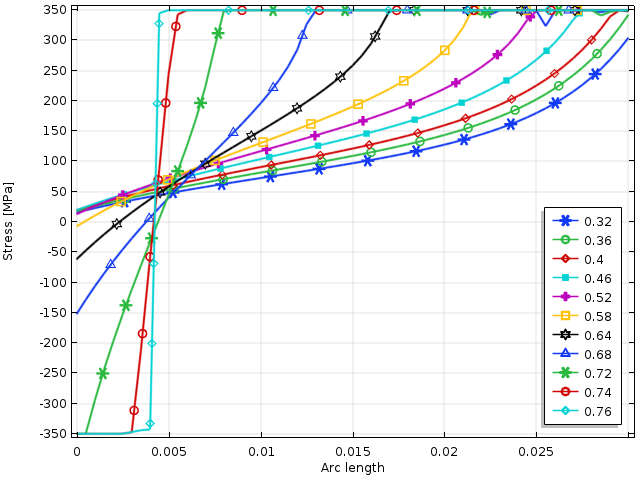
The stress distribution over a cross section as the external load is increased. The load parameter value is the ratio between the membrane stress and yield stress.
In this example, the values have been chosen so that σm = σb. Using the interaction formula above, this means that collapse should occur when
This value matches the final parameter value of 0.76 rather well. The difference can be explained by the fact that a small plastic hardening is used in the model to stabilize the analysis.
The conclusion is that for determining safety conditions within plastic collapse, the linearized stress is the relevant parameter, since it is proportional to the axial force and bending moment. Using the true peak stress gives an overly conservative design. The safety factor, which is implicit in the bending collapse, must also be taken into account.
If the structure is subjected to cyclic loading, the peak stresses are of utmost importance, as they determine the risk of fatigue crack initiation at the surface.
The ASME Pressure Vessel Code
The concept of stress linearization is an important part of the qualification of pressure vessels, as described in ASME Boiler & Pressure Vessel Code, Section III, Division 1, Subsection NB. Here, we are required to classify stresses as either primary or secondary.
A primary stress is a stress that is required for maintaining force and moment equilibrium. Secondary stresses are caused by other effects. Typically, secondary stresses are local effects caused by either geometric discontinuities or displacement-controlled loading. Secondary stresses do not lead to a collapse when they exceed elastic limits, since they are just redistributed.
During the analysis, the stress is studied along a number of lines through the section, referred to as stress classification lines (SCLs). The choice of SCL is not unique, so here we must use our engineering judgment to find the critical locations.
Although not fully correct (but conservative), the linearized stresses are sometimes viewed as equivalent to the primary stresses. Without going into detail, the basic requirements of the code are:
- The stress intensity (Tresca equivalent stress) from the primary membrane stresses should not exceed two-thirds of the yield stress. This gives a safety factor of 1.5 against plastic collapse when only membrane stresses are present.
- The stress intensity from the sum of membrane and bending stress should not exceed the yield stress. If there are only bending stresses, the safety factor against collapse is again 1.5. This is because incipient yield is not equal to the full collapse of the section in this case.
- Secondary stresses are allowed to reach twice the yield limit.
- There are similar requirements, but with higher safety factors against reaching the ultimate stress.
Interestingly enough, this means that if the membrane stress is at the limit allowed by the first criterion, it is still allowed to add a certain amount of bending stress. The discussion above tells us why: The bending stress reduces the stress over part of the section.
As noted above, the detailed stress state is not important when it comes to static failure, as the stress distribution in the collapse state is fully determined by the force and moment equilibrium. In the figure below, the collapse interaction curve is compared with the stress limits imposed by the code.
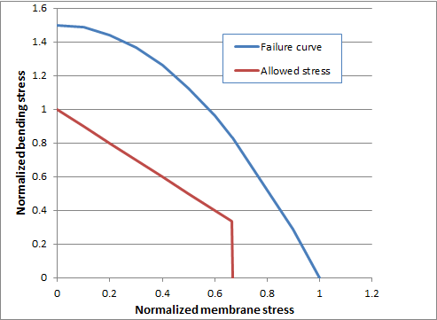
The fundamental ASME criteria for primary stresses. The stresses are normalized by the yield stress.
It should be noted that because pressure vessels often operate at elevated temperatures, room temperature values of allowed stresses might not be sufficient.
The requirement on the secondary stresses is set to avoid cyclic plastic deformation upon repeated loading–unloading cycles. The purpose is to avoid plastic strains accumulating in each load cycle, which can lead to a fast failure due to low-cycle fatigue.
Other Applications of Stress Linearization
Some rules for qualifying structural elements are based on the stresses being “hand calculated” or the result of a shell or plate analysis. When we do a full 3D analysis, the effect can be that we get results that are “too good”. The effects of local stress concentrations are already taken into account by providing low allowable nominal stresses. Because of this, we might end up in a situation where using the accurate results of a full 3D analysis leads to a highly conservative design. In this case, stress linearization can provide a useful tool for converting the 3D stress state back into a set of nominal stresses.
For instance, this situation can occur when analyzing welds. Typically, the local geometry at the weld is not even well defined (unless it is a very high-quality weld that has been ground smooth). Thus, the actual local stress is not even meaningful to compute, so we must resort to methods based on nominal stresses.
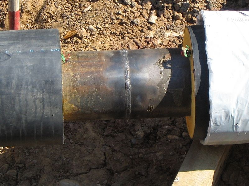
A weld in a pipe used for district heating. Image by Björn Appel, Benutername Warden. Licensed under CC BY-SA 3.0, via Wikimedia Commons.
Applying a Stress Linearization in COMSOL Multiphysics®
A stress linearization does not affect the analysis as such; it is a type of result presentation. The variables to be used are set up in the Solid Mechanics interface. We add a line for stress linearization either under Variables in the context menu for the Solid Mechanics interface or under Global on the Physics tab in the ribbon.
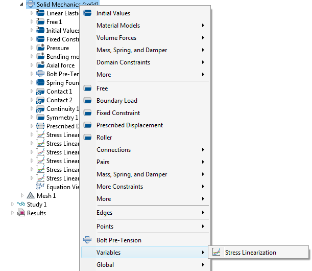
Adding a Stress Linearization node from the context menu.
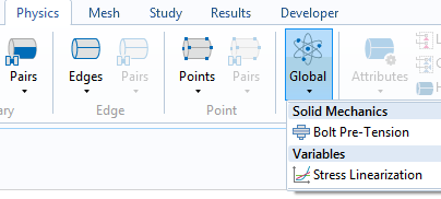
Adding a Stress Linearization node from the ribbon.
Depending on whether the component is in 3D or not, the definition of the stress linearization line comes in two different flavors. In either case, we select an edge (or set of edges) that forms a straight line through the thickness of the component that we are evaluating. In 3D, we must also define the axis orientation of the local coordinate system in which the stresses along the SCL are represented.
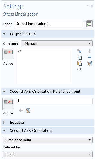
The settings for stress linearization in 3D.
The stress tensor components along an SCL are represented in a local coordinate system, where 1 is the direction along the line. The 2 direction is perpendicular to the line and has the following orientations:
- In the plane of a 2D model
- In the hoop direction of a 2D axially symmetric model
- Along a user-specified direction for a 3D model
For the last bullet point, note that the Second Axis Orientation section of the Stress Linearization node provides several options for entering the orientation.
If we have defined the SCLs prior to the analysis, then one edge data set is generated for each SCL. At the same time, a default plot called Stress Linearization is added.
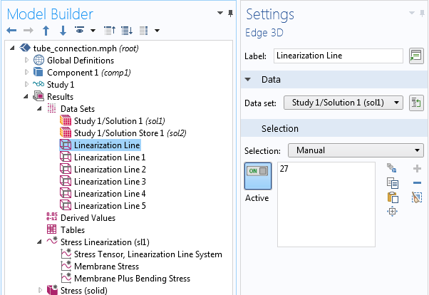
The default data sets and graph plot group.
The stress linearization plot contains three graphs along the selected SCL:
- Actual stress
- Membrane stress
- The sum of the membrane and bending stress
An example of a default stress linearization plot.
In the stress linearization plot, we can change to another SCL by selecting the corresponding edge data set. In the default plot, the 22 stress tensor component is displayed. Of course, we can change to other components. Usually, 33 and 23 are the most important.
If we add Stress Linearization nodes after running the analysis, we must click on the Update Solution button to make the newly created variables accessible for result presentation. No default plots or data sets are automatically generated in this case.
Graphing along the SCLs is important for understanding the stress state at different locations, but at the end of the day, it is the stress intensity that is important. The maximum stress intensity for each SCL can be presented by adding a Global Evaluation node. When computing the stress intensity for the bending stress plus the membrane stress, the bending part of the out-of-plane stress components (which are supposedly small) is ignored. This approach is customary in this type of analysis.
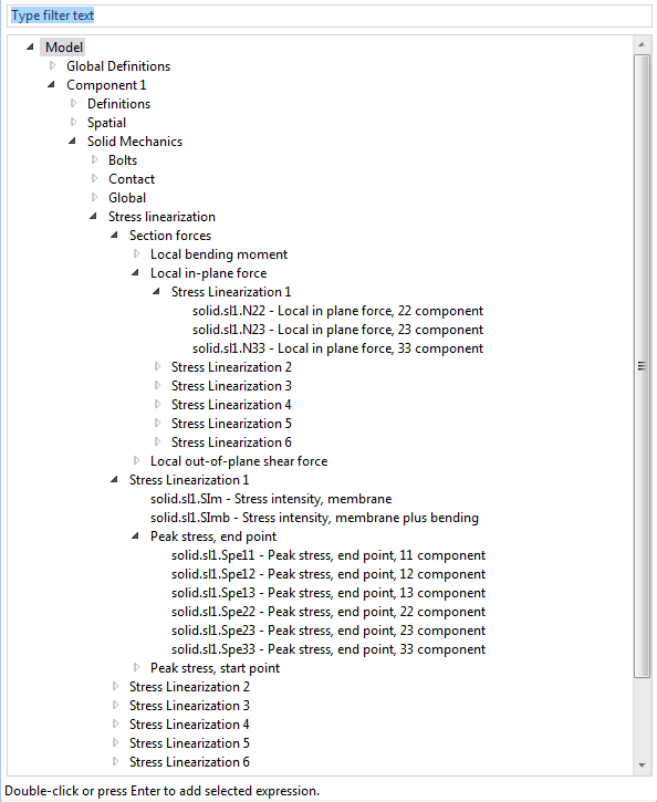
The result quantities for stress linearization when selecting data for a Global Evaluation node.
In addition to the stress intensities, the peak stress tensor at the two ends of the SCL is available. We can also directly access the section forces and moments corresponding to the linearized stresses.
Final Remarks on Performing a Stress Linearization in the Structural Mechanics Module
As of version 5.3 of COMSOL Multiphysics® and the Structural Mechanics Module, the functionality for stress linearization provides us with a set of built-in tools for converting a 3D stress state to one of pure bending and tension. This makes it much easier to produce results that comply with various design codes.
Further Resources
- Learn more about structural analysis in these blog posts:
- Watch this video for an introduction to modeling structural mechanics


Comments (0)