Aeroacoustics
The Interaction Between a Background Flow and an Acoustics Field
The generation of sound by a turbulent flow is the most common physical effect associated with the field of aeroacoustics. The prefix aero means air, however, the field of aeroacoustics is not restricted to flow-induced noise in air. Aeroacoustics is concerned with the general interaction between a background flow and an acoustics field. For example, if you were studying the reflections of sound off a shear layer or how the flow in a muffler affects transmission loss, you would be studying aeroacoustics.
Aeroacoustics models can include effects that alter an acoustic field in the presence of a flow, such as turbulence, local variations in material properties, convection, viscous damping, and much more. Numerically solving aeroacoustic problems falls under the field of computational aeroacoustics (CAA).
Flow-Induced Noise
Acoustic noise generated by a flow can be created through different mechanics, but is ultimately due to fluctuations in the flow. These fluctuations will give rise to distributed acoustic sources throughout the flow. Noise is created by local stress fluctuations in the flow (Reynolds stresses, viscous stress effects, and nonisentropic effects all act as quadrupole sources); pressure fluctuations at walls (e.g., dipole sources at solid boundaries); mass and heat fluctuations (e.g., distributed monopole sources); and external fluctuating force fields.
Acoustic waves are only a subset of waves that are created by the flow; vorticity and thermal instability waves are also produced. These particular waves are only convected by the flow, whereas acoustic waves also propagate relative to the flow, at the local speed of sound. Compared to other fluctuations, the energy associated with acoustic waves is typically many orders of magnitude smaller. This means that a direct simulation of the flow-induced noise is very challenging and requires extremely accurate numerical schemes. Another difficulty is that the acoustic sources occur at the length scale of the turbulence in the flow, which then needs to be resolved.
Acoustic Analogies
Acoustic analogy equations are formulations that separate out acoustic fluctuations from flow fluctuations.
The first form of these equations derived from the seminal work of J. Lighthill in the 1950s. His acoustic analogy equation is obtained by rearranging the Navier-Stokes equations, which result in a convected scalar wave equation for the acoustic pressure and a right-hand side that contains all of the flow source terms.
Analogy equations can also be constructed by rearranging the flow equations in other ways, leading to linearized Euler equations or linearized Navier-Stokes equations with right-hand side flow sources. The linearized models have great applicability in many aeroacoustics situations where the flow-induced noise is not important. This is found in fluid-structure interaction (FSI) problems in the frequency domain, when modeling how a background flow affects the acoustics (e.g., reflection and refraction), detailed muffler models, and much more.
Linearized Models of Aeroacoustics
Ideally, aeroacoustic simulations would involve solving the fully compressible Navier-Stokes equations in the time domain. Acoustic pressure waves would then form a subset of the fluid solution. However, this approach is often impractical for real-world applications, due to the computational time and memory resources required.
Instead, like solving for many practical engineering problems, a decoupled two-step multiphysics approach is used:
- Solve for the fluid flow
- Solve for the acoustic perturbations on top of the flow
Several models exist that include different levels of detail and different aeroacoustic effects. These models are derived by linearizing the dependent variables around a steady-state background flow and making physical assumptions. The dependent variables now represent perturbations, such as acoustic and instability waves, on top of the flow. The classical scalar wave equation, otherwise known as the Helmholtz equation in the frequency domain, is an example of a linearized model with no explicit losses and an isentropic assumption.
Types of Linearized Models
Scalar Wave Equation
In its general form, the scalar wave equation includes the dependency of the speed of sound and density on the background flow (as they can both be spatially varying). It is a good approximation when convective effects are not important (i.e., when the Mach number is less than 0.1) and thermal and viscous losses are also negligible.
Thermoacoustics
Linearized thermoacoustics models involve the dependency of material parameters on the background flow, as well as thermal and viscous losses. They are sufficient models when the Mach number is less than 0.1. An application example is modeling FSI in the frequency domain.
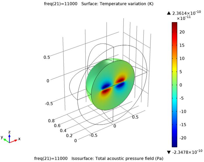
Model of a vibrating micromirror. The plot shows the acoustic variations of the temperature field.
Model of a vibrating micromirror. The plot shows the acoustic variations of the temperature field.
Linearized Potential Flow
Linearized potential flow models involve the interaction between a background potential flow and the acoustic field. Here, no losses are modeled except for possible impedance conditions at walls. Linearized potential flow can be used for modeling sound propagation from jet engines, for example.
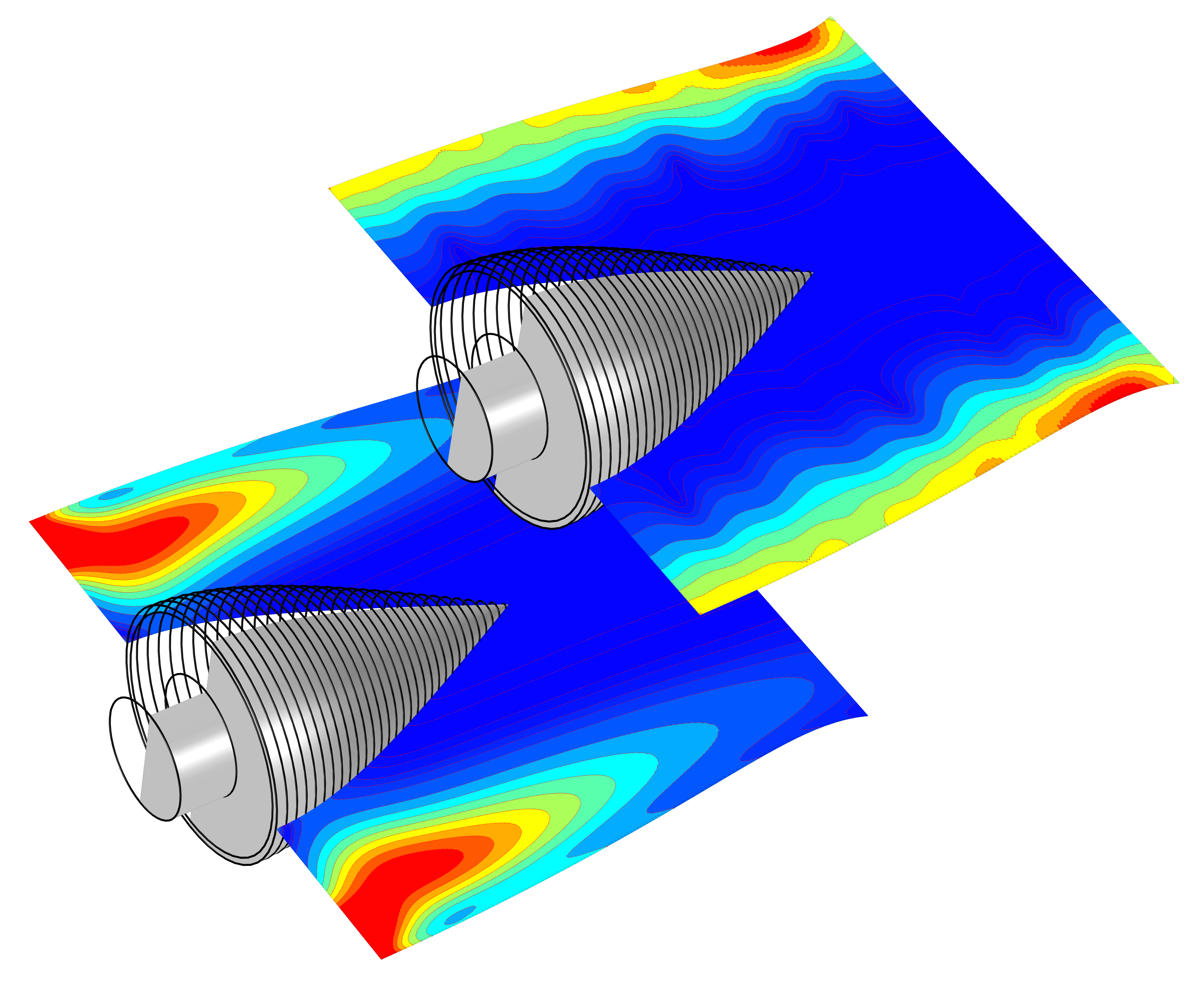
Acoustic pressure distribution on a lined duct wall of a jet engine.
Acoustic pressure distribution on a lined duct wall of a jet engine.
Linearized Euler
Linearized Euler models can be used to compute acoustic variations in density, velocity, and pressure in the presence of a stationary background mean flow that is well approximated by an ideal gas flow. In its general form, this equation supports both acoustic and nonacoustic waves. The latter are so-called instability waves (vorticity and entropy waves).
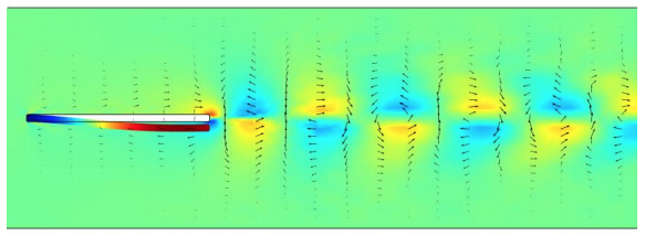
Visualizing the vibrations of a plate in a 2D viscous parallel plate flow. Modeled with the linearized Navier-Stokes equations.
Visualizing the vibrations of a plate in a 2D viscous parallel plate flow. Modeled with the linearized Navier-Stokes equations.
Linearized Navier-Stokes
Linearized Navier-Stokes equations are used to compute the acoustic variations in pressure, velocity, and temperature in the presence of any stationary isothermal or nonisothermal background mean flow. These equations include viscous losses, thermal conduction, and heat generated by viscous dissipation, if relevant.
Acoustic Perturbation Equations
There are many variations and modifications of the aforementioned linearized models for modeling aeroacoustics problems. One such example is the acoustic perturbation equations. Here, nonacoustic propagating modes have been filtered out by modifying the governing equation, resulting in a pure acoustic problem.
Published: September 28, 2015Last modified: February 21, 2017