Response Spectrum Analysis
What Is Response Spectrum Analysis?
Response spectrum analysis is a method to estimate the structural response to short, nondeterministic, transient dynamic events. Examples of such events are earthquakes and shocks. Since the exact time history of the load is not known, it is difficult to perform a time-dependent analysis. Due to the short length of the event, it cannot be considered as an ergodic ("stationary") process, so a random response approach is not applicable either.
The response spectrum method is based on a special type of mode superposition. The idea is to provide an input that gives a limit to how much an eigenmode having a certain natural frequency and damping can be excited by an event of this type.
The text below is separated into three parts:
- The definition of a response spectrum
- Generation of a response spectrum from a given time history
- The use of a given response spectrum in a structural analysis
In most cases, the engineer performing a response spectrum analysis is presented with a given design response spectrum, in which case the two first parts can be considered as background material.
Definition of a Response Spectrum
A response spectrum is a function of frequency or period, showing the peak response of a simple harmonic oscillator that is subjected to a transient event. The response spectrum is a function of the natural frequency of the oscillator and of its damping. Thus, it is not a direct representation of the frequency content of the excitation (as in a Fourier transform), but rather of the effect that the signal has on a postulated system with a single degree of freedom (SDOF).
Analysis of an SDOF System
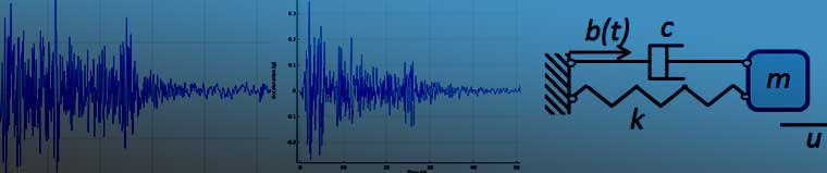
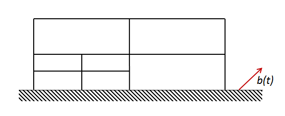
Consider a mass-spring-damper system attached to a moving base. The foundation has a given movement,  .
.
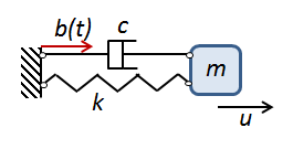 The SDOF system.
The SDOF system.
The SDOF system.
The equation of motion for the mass can, if there are no external forces, be written as

Dividing by the mass, and using customary notation,

Here, the undamped natural (angular) frequency is

and the damping ratio is

It can be seen that the support movement acts as a forcing term and that the solution depends only on the two parameters  and
and  , but not on the individual values of m, c, and k.
Instead of using the absolute displacement as the degree of freedom, it is possible to choose the relative displacement between the mass and the base,  . This is actually a frame transformation where the oscillator is studied in a coordinate system attached to the base. As in any accelerating frame, there will be inertial forces. The equation of motion can be stated as
 (1)
(1)
Thus, the support acceleration appears as a gravity-like load. There are two advantages with this representation:
- The internal forces in the system — that is, elastic and damping forces — depend on relative displacements and velocities. These forces are not affected by a rigid body motion.
- Often, measured data is available in terms of an accelerogram, so that the foundation displacements are not directly available.
For given values of , , and , this equation can be solved for a sufficiently long time. The displacement, velocity, and acceleration response spectra are defined as the maximum values caused by the acceleration history .


These are all relative spectra. It is possible to do a similar definition of the absolute spectra, by instead using the absolute displacement  .
.
Sometimes, a distinction is made between the positive and negative spectra, so that


and similarly for velocity and acceleration spectra.
The velocity and acceleration response spectra are often approximated by


Such spectra are called pseudovelocity and pseudoacceleration spectra.
For a system without damping, the pseudoacceleration spectrum based on the relative displacement is actually equal to the absolute acceleration spectrum. This can be seen from the undamped equation of motion,

Thus,

The maximum absolute value of the relative displacement must thus occur at the same time as the maximum absolute value of the absolute acceleration. The scale factor between the two is  . For systems with low damping, this relation will still be approximately true. Since most mechanical systems have a low damping (often 2% to 5%), it is customary to assume that the spectra for the absolute acceleration and the pseudoacceleration are the same.
Another common way of describing the damping in this context is by the Q factor (quality factor). The relation to the damping ratio is given by

How to Create a Response Spectrum
For a certain given time history, , a response spectrum is created in the following way:
- Select a frequency range for which the spectrum should be generated
- Select a frequency step that determines how many points on the response spectrum should be computed
- Select a certain damping ratio,
- For each of the selected frequencies
a. Solve Equation (1) with for a sufficiently long time
b. Keep track of the maximum value of and store it
The equation can be solved by a pure numerical time stepping, but there may be better ways of doing it. If  is given as a number of points in an accelerogram, then it is natural to assume that the acceleration has a linear variation in time between those points. So, for each interval between two measurements, say from
  to
to  , the equation of motion for the oscillator is

This equation, where the right-hand side is a linear function of time, can be solved analytically for each time interval. The initial conditions are obtained from the final state of the previous interval.
The maximum values can actually occur after the end of the driving event. This will happen for low values of (long periods). The time-stepping must thus be continued at least until a full period if the oscillator has elapsed.
With this formulation, it is possible to track the extreme values of the:
- Relative displacement
- Relative velocity
- Relative and absolute acceleration
The absolute displacement and velocity are not available, since only is known, but not  and
and  . It is, of course, possible to recover the foundation velocity and displacement by time integration of the acceleration. In practice, this integration will, however, cause a drift, so that the final velocity and displacement turn out to be nonzero. Since nonzero final displacements and velocities are unphysical (at least for many types of events), some numerical filtering has to be applied. For shocks, there is also a question of which initial values should be chosen for the displacement and velocity of the foundation.
Example 1: A Half Sine Shock
A common description of impact, used in several standards, is a half sine acceleration pulse. The acceleration amplitude, as well as the duration of the shock, can have different values. The acceleration may, for example, be 20 g, 50 g, or 100 g (g = 9.8 m/s2), and the time of duration can be 6 ms or 11 ms. In this example, a 50-g half sine pulse with a duration of 11 ms is used as the acceleration .
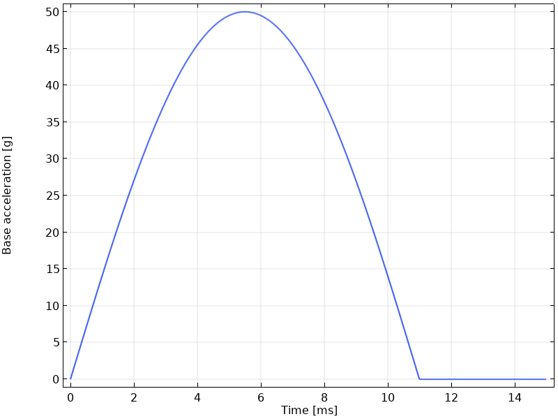 The base acceleration for the 50-g, 11-ms half sine shock.
The base acceleration for the 50-g, 11-ms half sine shock.
The base acceleration for the 50-g, 11-ms half sine shock.
The computed response spectra for 5% damping (Q = 10) is shown below.
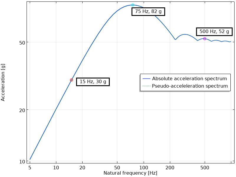 The absolute acceleration response spectrum for 5% damping plotted together with the corresponding pseudoacceleration spectrum.
The absolute acceleration response spectrum for 5% damping plotted together with the corresponding pseudoacceleration spectrum.
The absolute acceleration response spectrum for 5% damping plotted together with the corresponding pseudoacceleration spectrum.
The absolute acceleration has a maximum at frequencies similar to the frequency content of the input signal. In this case, the peak is at 74 Hz (T = 13.5 ms). For high frequencies, the acceleration spectrum tends toward 50 g. This is a general observation for any signal: At high frequencies, the oscillator will behave as a rigid body, so the mass just follows the base motion. As an effect, the asymptotic value of the absolute acceleration spectrum always equals the peak base acceleration during the event.
For low frequencies, the acceleration tends toward zero with a rate that is inversely proportional to the frequency. With a very soft oscillator, the base movement will just compress the spring without significant movement of the mass.
It can also be seen that the pseudoacceleration spectrum in this case is almost indistinguishable from the actual absolute acceleration spectrum, even though the damping is 5%.
In the figures below, the time response for the oscillator is shown for three different choices of its natural frequency, corresponding to the markers in the response spectrum above.
- At 15 Hz, the load pulse just gives a small initial push, and then the oscillator experiences free vibration at its natural frequency. The peak acceleration occurs a long time after the end of the excitation.
- At 75 Hz, there is maximum dynamic amplification. The load pulse is essentially in phase with the relative velocity, and it provides a maximal energy input to the system.
- At 500 Hz, the oscillator to a large extent acts as a rigid body, closely following the base acceleration. The peak acceleration is almost the same as that of the base acceleration.
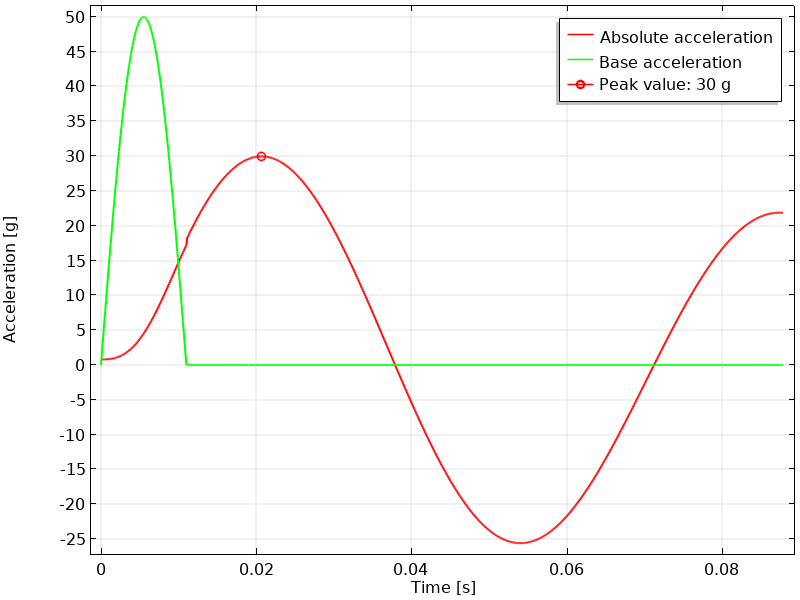 Absolute acceleration at a natural frequency of 15 Hz and damping of 5%.
Absolute acceleration at a natural frequency of 15 Hz and damping of 5%.
Absolute acceleration at a natural frequency of 15 Hz and damping of 5%.
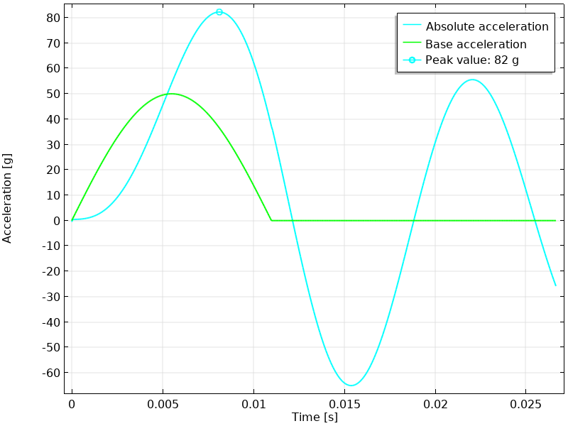 Absolute acceleration at a natural frequency of 75 Hz and damping of 5%.
Absolute acceleration at a natural frequency of 75 Hz and damping of 5%.
Absolute acceleration at a natural frequency of 75 Hz and damping of 5%.
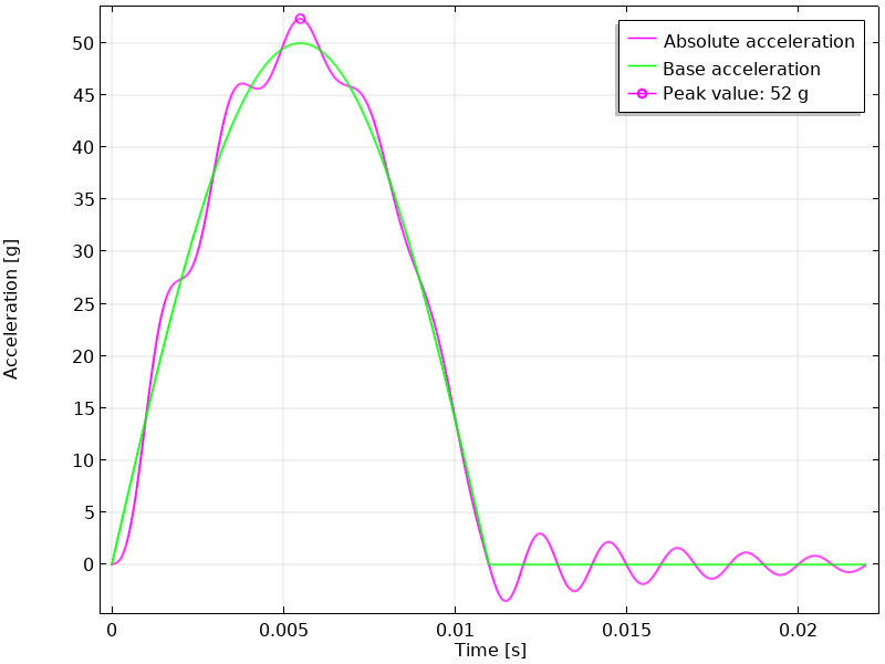
Absolute acceleration at a natural frequency of 500 Hz and damping of 5%.
Absolute acceleration at a natural frequency of 500 Hz and damping of 5%.
The relative displacement spectrum is shown below. This is essentially the same as the acceleration spectrum above, but scaled with a factor 
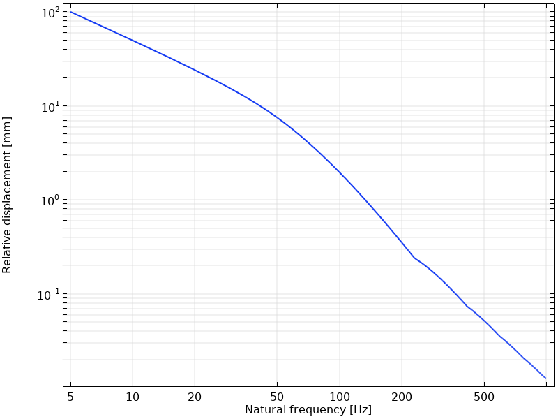 The relative displacement response spectrum for 5% damping.
The relative displacement response spectrum for 5% damping.
The relative displacement response spectrum for 5% damping.
Next, the relative velocity spectrum and the pseudovelocity spectrum are compared. As can be seen, they are quite different. The pseudovelocity and pseudoacceleration spectra do not represent the true relative spectra. This is a general observation, and the pseudo spectra should be viewed as different representations of the displacement spectrum.
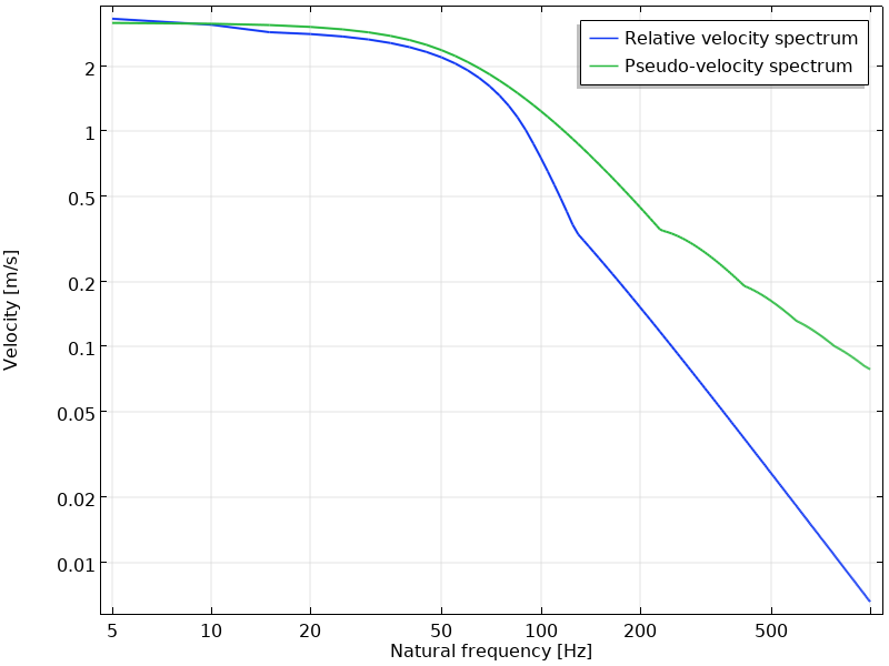 The relative velocity response spectrum and the pseudovelocity spectrum for 5% damping.
The relative velocity response spectrum and the pseudovelocity spectrum for 5% damping.
The relative velocity response spectrum and the pseudovelocity spectrum for 5% damping.
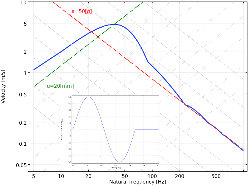
A convenient way to represent a response spectrum is in a tripartite, or four-axis plot. In such plot, the relative displacement, pseudovelocity, and pseudoacceleration are shown simultaneously. This is possible, since they are related by a factor of frequency and frequency squared, respectively, which in a logarithmic plot just gives lines with different slopes. The tripartite plot is essentially a pseudovelocity plot but with two extra sets of skewed grid lines that represent the displacement and acceleration, respectively.
 Tripartite plot of the response spectrum for the half sine pulse. The 50-g acceleration level and 20-mm displacement level are highlighted in red and green, respectively. The diagonal displacement (dotted) and acceleration (dashed) levels have the same '1-2-5-10' spacing as used for the velocity axis.
Tripartite plot of the response spectrum for the half sine pulse. The 50-g acceleration level and 20-mm displacement level are highlighted in red and green, respectively. The diagonal displacement (dotted) and acceleration (dashed) levels have the same '1-2-5-10' spacing as used for the velocity axis.
Tripartite plot of the response spectrum for the half sine pulse. The 50-g acceleration level and 20-mm displacement level are highlighted in red and green, respectively. The diagonal displacement (dotted) and acceleration (dashed) levels have the same '1-2-5-10' spacing as used for the velocity axis.
The response spectrum for the half sine pulse is actually somewhat atypical. The reason is that this pulse only has positive acceleration. If it is integrated with respect to time, such pulse corresponds to a resulting nonzero velocity and an ever-increasing displacement. Most events, like earthquakes, have the property that both displacement and velocity are zero both before and after the event. If a complete sine pulse is used instead of a half sine pulse, the characteristic low-frequency decay is also obtained.
 Response spectrum for a full sine pulse.
Response spectrum for a full sine pulse.
Response spectrum for a full sine pulse.
Example 2: The El Centro Earthquake
One of the most studied earthquake recordings is that of the "El Centro" earthquake on May 18, 1940. Recorded signals (with some filtering) are shown below.
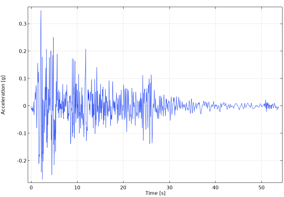
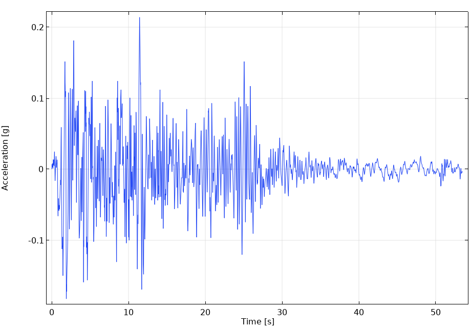
Acceleration in the N–S direction (left) and E–W direction (right) for the El Centro earthquake. Strong-motion data accessed through the Center for Engineering Strong Motion Data (CESMD). The networks or agencies providing this data are the California Strong Motion Instrumentation Program(CSMIP) and the USGS National Strong Motion Project(NSMP).*
These curves are typical for an event for which response spectrum analysis is relevant. A visual examination of the signal suggests that the main frequency content is in the range of 1–3 Hz, while the duration of the major part of the event is about 30 s. Thus, the conditions are not even close to being considered as a steady state. On the other hand, there is a significant number of cycles (of the order of 100), which can excite a structure having resonances in the 0.5–30-Hz range.
The computed response spectra for 2% and 5% damping are shown below.
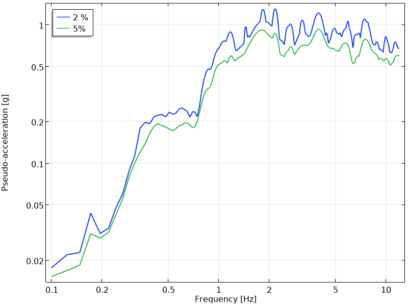 Pseudoacceleration spectra for the N–S direction for the El Centro earthquake.
Pseudoacceleration spectra for the N–S direction for the El Centro earthquake.
Pseudoacceleration spectra for the N–S direction for the El Centro earthquake.
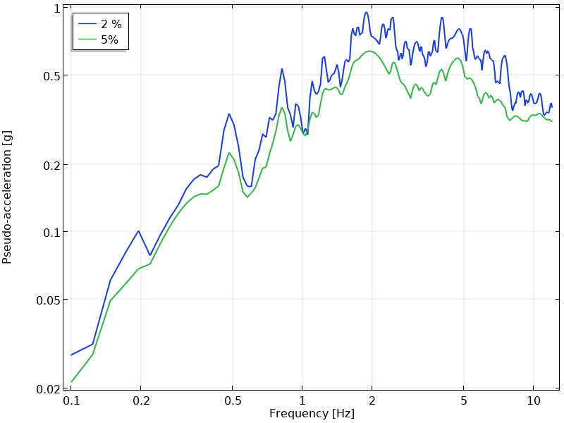 Pseudoacceleration spectra for the E–W direction for the El Centro earthquake.
Pseudoacceleration spectra for the E–W direction for the El Centro earthquake.
Pseudoacceleration spectra for the E–W direction for the El Centro earthquake.
The response spectra exhibit some interesting general properties. Higher damping will give lower response values and a smoother spectrum. Both these properties are related to the fact that the frequency response of an oscillator will have lower but wider peaks at higher damping.
Furthermore, there is a significant difference in the amplitudes in the N–S and E–W directions. However, there is a general resemblance between the shapes of the spectra in the two directions.
Design Response Spectra
The response spectrum of a single time signal is seldom of interest for an analysis, since it would be better to perform a direct time domain analysis of the structure with the original signal as input. As seen in the El Centro example above, a certain earthquake may give a response spectrum with significant peaks at certain frequencies. The peaks for another similar earthquake may, however, be located at other frequencies.
In order to be able to use a response spectrum for analysis of an event that has not yet happened, a design response spectrum is created. The design response spectrum can be seen as an envelope over all known and anticipated earthquakes in a certain geographical region. Such spectra are, for example, provided in building codes like ASCE 7-16 and Eurocode 8 (Ref. 2–3). The acceleration levels in a design response spectrum will typically depend on the geographical location and the type of soil.
The design response spectrum is the actual input to the response spectrum analysis.
Design response spectra are often provided in terms of the period, rather than the frequency. Since one is the inverse of the other, the two graphs are just mirrored when plotting on a logarithmic scale.
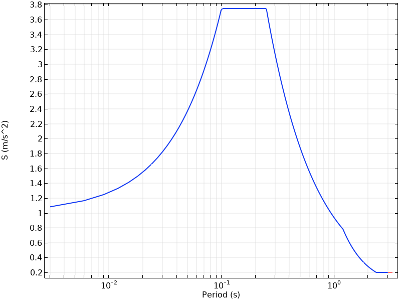 Example of a design response spectrum.
Example of a design response spectrum.
Example of a design response spectrum.
Floor Response Spectrum
A typical design response spectrum for earthquakes gives information about the effect of the ground motion on a primary structure like a building. However, if we are interested in analyzing a secondary component or system that is mounted inside the building, the original response spectrum may not provide a suitable description. The secondary system can, for example, be a piping system or a pressure vessel. The secondary system will be subjected to a base acceleration at its location inside the primary structure. This acceleration is, in general, not the same as the acceleration of the ground.
A floor response spectrum is a type of design response spectrum developed for a certain location in a primary structure. The primary structure will, through its natural frequencies, act as a bandpass filter for the original signal. Thus, the floor response spectrum will typically have significant peaks related to the natural frequencies of the primary structure. The term floor response spectrum is derived from the fact that this local response spectrum will typically be different between different floors of a building.
A large system, like a piping system, may not have the same floor response spectrum at all of its support points. This causes significant complications to the analysis.
Analysis Based on Response Spectra
The Multiple DOF System
Assume that a mathematical model of a structure is discretized by FEM so that the equations of motion on matrix form are 
The structure is at a number of points connected to a common "ground" that has the base motion  . This vector has the same size as
  (the total number of DOFs), but it contains only three different values:
  in all x-translation DOF,
  in all y-translation DOF, and
  in all z-translation DOF. The relative displacement is now
  . With no external load, the equation of motion is

or

Here, the fact that a rigid body motion does not introduce any elastic or viscous forces in the system has been used, so that  .
.
By solving the undamped eigenvalue problem  with the support nodes being fixed, a set of N eigenmodes

can be computed.
These eigenmodes can represent the relative displacements (but not the absolute displacements), since all eigenmodes will have zero displacements at the support points in an eigenfrequency analysis.
By standard operations for mode superposition, the decoupled modal equations are

It has been assumed that the mass matrix normalization of the eigenmodes is used and that the damping matrix can be diagonalized by the eigenmodes. The mass matrix normalization is not essential, but it will simplify certain expressions.
Here,  is the modal coefficient for mode j, so that the relative displacement can be written as a linear combination of eigenmodes, weighted by the modal coordinates:

The support motion can be decomposed along three orthogonal directions as

The vector  has the value "1" in all X-translation DOFs and the value "0" in all other. The modal equation of motion is then

The multipliers  are the modal participation factors;

Thus, the maximum amplitude of mode j, when loaded by a base motion in direction k described by a response spectrum, is

or, using the pseudoacceleration spectrum

To summarize, the peak amplitude for a certain eigenmode is the product of the response spectrum value at the corresponding natural frequency (which is independent of the structure) and the participation factor (which is a property of the structure but independent of the loading).
Summation Over Modes
In practice, several modes will have natural frequencies in the frequency range covered by the design response spectrum. This means that some combination of their responses is needed. There are several rules for how this combination can be arranged, as will be described in detail below.
These summation rules are nonlinear. For all combination types, all result quantities are strictly positive. As an effect, any quantity must be summed based on its own modal response. For example, stress components must be computed using the modal stresses and cannot be recovered from the summed strains, and strains cannot be recovered from summed displacements. This has many consequences for the interpretation of results from a response spectrum analysis. Some examples are:
- It is not meaningful to plot displacement shapes, since the individual displacement components do not match.
- An equivalent stress, like von Mises, cannot be computed from individual stress components.
- If there are interaction rules, like the combination of normal force and moment in a beam, the way of doing the summation is sensitive. A conservative interpretation separately determines the two quantities and then works with the sums and differences.
- Particular care must be taken with respect to the signs if the results of the response spectrum analysis are to be added to results from a static load case, like a dead load.
Often, the excitation is given in three orthogonal directions. The general approach is to consider the excitation in the three directions  separately. First, all modal responses are summed for each direction, and then the results for the three directions are summed. An exception is the CQC3 summation rule, described below, in which the spatial and modal summation is done at the same time.
Periodic and Rigid Modes
It is often useful to divide the eigenmodes into periodic modes and rigid modes. The distinction is related to the frequency content of the excitation relative to the eigenfrequency of the mode.
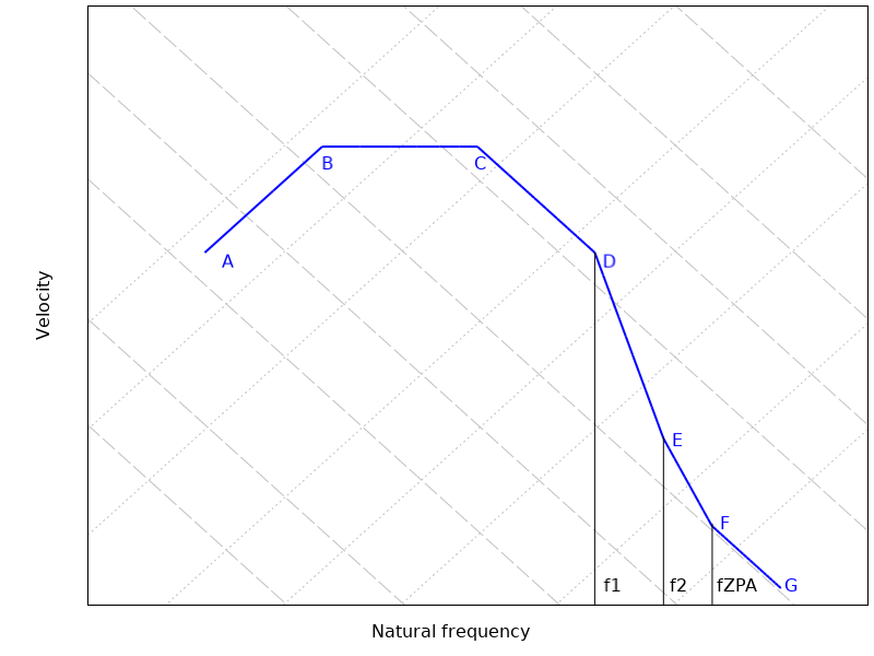 A characteristic design response spectrum based on NRC RG 1.92 (Ref. 1)
A characteristic design response spectrum based on NRC RG 1.92 (Ref. 1)
A characteristic design response spectrum based on NRC RG 1.92 (Ref. 1)
In the response spectrum above, the following characteristic domains can be identified:
| Region | Description | Response Type |
|---|---|---|
| A-B | Amplified periodic spectral displacement | Periodic |
| B-C | Amplified periodic spectral velocity | Periodic |
| C-D | Amplified periodic spectral acceleration | Periodic |
| D-E | Transition from amplified periodic spectral acceleration to rigid spectral acceleration | Mix of periodic and rigid |
| E-F | Transition from rigid spectral acceleration to maximum base acceleration | Rigid |
| F-G | Maximum base acceleration | Rigid |
The table above is based on NRC RG 1.92 Ref. 1.
In a high-frequency mode, the mass of the oscillator will mainly be translated in phase with the support. Such modes constitute the rigid modes. Their responses are synchronous with each other (and with the base motion). This means that for rigid modes, a pure summation (including signs) should be used.
Modes with a significant dynamic response constitute the periodic modes. The maximum values for such modes will be more or less randomly distributed in time, since their periods differ. For this reason, the periodic part of the response requires more sophisticated summation techniques. A plain summation of the maximum values will, in general, significantly overestimate the true response.
Modes that are in a transition region will partially contribute to the periodic modes and partially to the rigid ones. In addition, it is sometimes necessary to add some static load cases containing a missing mass correction.
Not all analyses require a separation into periodic and rigid modes. If not, all modes are treated as periodic.
In the following,  denotes any result quantity caused by excitation in direction
  . can be, for example, displacement, velocity, acceleration, a strain component, a stress component, effective stress, or a beam section force. The periodic part of is denoted
  , and the rigid part is denoted
  . Similarly,
  and
and  denote the results from an individual eigenmode j.
Partitioning into Periodic and Rigid Modes
There are two different methods in use by which partitioning can be done. In either case, for mode j,


so that

The difference between the two methods lies in how the coefficient  is determined. For low frequencies, it should approach the value 0, and for high frequencies, the value 1.
Gupta Method
In the Gupta method, is a linear function of the logarithm of the natural frequency.


Here,  and
and  are two key frequencies. Thus, for eigenfrequencies below , the modes are considered as purely periodic, and above , purely rigid. In the original Gupta method, the lower key frequency is given by

Here,  and
and  are the maximum values of the acceleration and velocity spectra, respectively. In the idealized spectrum above, this occurs at the point D.
The second key frequency should be chosen so that the modes above this frequency behave as rigid modes. The frequency can be taken as the one where the response spectra for different damping ratios converge to each other.
Lindley-Yow Method
In the Lindley-Yow method, the coefficient depends directly on the response spectrum values, not only on the frequency. As a consequence, it is possible that a certain mode can be considered as having a different degree of rigidness for different excitation directions.

The so-called zero period acceleration (ZPA) is the maximum ground acceleration during the event,

This is also the high-frequency asymptotic value of the absolute acceleration (or pseudoacceleration) in the response spectrum. It corresponds to the F-G part of the idealized spectrum.
Thus,

The value of must, for physical reasons, be in the range of 0 to 1 and increase with frequency. For this reason, NRC RG 1.92 (Ref. 1) requires that be set to zero for any eigenmodes below point C.
Summing the Periodic and Rigid Modes
Once the periodic and rigid responses for all modes have been summed up separately, they are combined as

Summing the Periodic Modes
Absolute Sum Method
The most conservative method is to sum the maximum response for all N modes, thus assuming that all modes reach their maximum at the same time. In many cases, this approach leads to a design that is significantly overconservative.

In the worst case scenario, the predicted result using N, not closely spaced modes can be a factor  larger than what would be obtained using the other methods below.
Complete Quadratic Combination
The most popular method for superposition of the periodic modes is the complete quadratic combination (CQC) method:

The interaction between the modes is determined by the mode interaction coefficient  (
( ). Since is symmetric and
  when
when  , it is more efficient to use the equivalent expression

This expression is actually valid for several evaluation rules. The only difference is how is computed. Several such expressions are given below. When a method is referred to as CQC, it is usually implied that the Der Kiureghian correlation coefficient is used.
Der Kiureghian Correlation Coefficient
The mode interaction coefficient is defined as

Here,  and
and  are the natural frequencies of the two modes, and
  and
and  are the corresponding modal damping ratios.
For the common case of uniform damping, the expression can be simplified to

It is possible that the response from two different modes,  and , have different signs, so that a cross term can give a negative contribution to the sum. This is intentional, but it is a common misconception that the absolute values of and should be used. However, the underlying analysis contains an assumption about the response being a linear function of the mode shape. If this it not the case, using absolute values is a safer approach. The most common nonlinear result quantities, like effective stresses, are always positive, in which case all terms in the sum will give a positive contribution anyway.
The strength of the correlation between two modes depends on the frequency ratio for the modes, but it also strongly depends on the damping.
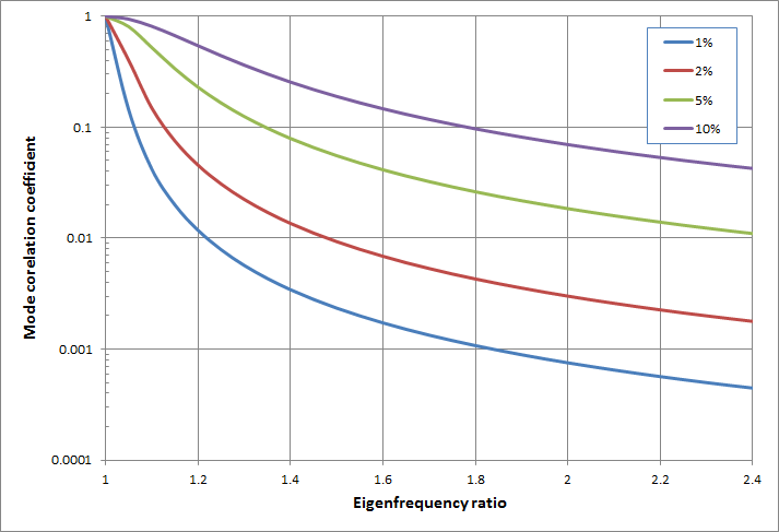 The Der Kiureghian mode correlation factor for different damping ratios as a function of the ratio between the pair of eigenfrequencies.
The Der Kiureghian mode correlation factor for different damping ratios as a function of the ratio between the pair of eigenfrequencies.
The Der Kiureghian mode correlation factor for different damping ratios as a function of the ratio between the pair of eigenfrequencies.
Double Sum Method
The double sum method uses a mode interaction coefficient  , which is called the Rosenblueth correlation coefficient. It is conceptually similar to the Der Kiureghian correlation coefficient.
The double sum method exists in two variants:

(NRC Regulatory Guide 1.92, rev 1)
(NRC Regulatory Guide 1.92, rev 2, 3)
The older version of this method is actually erroneous, but the results are more conservative than those of the newer variant, so it can be used without risk.
In either case,

where

and

Here,  is a separate input. The duration of the dynamic event and are the modal damping ratios. For large values of , the modal correlation factor in the double sum method is rather similar to that of the Der Kiureghian model. For smaller values of , a much stronger correlation is predicted by the double sum method.
SRSS Method
The SRSS method does not include any interaction between the modes; that is,


This method should only be used when the modes are not closely spaced; that is, when no two eigenfrequencies are close to each other. All other methods take possible interaction between the modes into account in various ways.
Grouping Method
The modes are grouped according to the following rule:
- Start a new group by adding the lowest (in frequency), not yet grouped eigenmode k
- Step up through the eigenfrequencies from k
- As long as
 , add mode i to the group
 - Go back to Step 1
After having exhausted the list of eigenmodes, there is a number of groups, where some may contain just a single eigenmode. The rule for the correlation factor between two modes is


The sign() operator used here is a way of stating that the absolute value of the product of the modal responses is added to the sum, since

Ten Percent Method
The ten percent method is similar to the grouping method in the sense that eigenmodes with a natural frequency difference of less than 10% get a special interaction treatment. The modal correlation coefficient is


It can be noted that both the grouping method and the ten percent method are equivalent to the SRSS method if no pair of eigenfrequencies are within 10% from each other. When using the CQC method, however, the modes are also considered as significantly coupled at a larger spacing, unless the damping is very low.
Summing the Rigid Modes
There are two possible combination methods for summing the rigid modes.
Combination Method A
The rigid modes are summed as

Here,  is the result of the solution to the static load case when solving for missing mass, as described below.
Combination Method B
This method can only be used when the Lindley-Yow method is used together with the static ZPA method. Then, the rigid mode response is simply

Missing Mass Correction
Missing Mass Method
Since a mode superposition uses a limited number of modes, some mass that is attributed to the nonused modes will, in general, be missing from the analysis. With the assumption that the higher-order modes do not have any dynamic amplification, it is possible to devise a correction by solving some extra static load cases containing the peak acceleration acting on the "lost" mass. The effect of applying a static correction is usually most prominent when evaluating support forces.
So-called static correction can actually be used for mode superposition in general. However, for the case of response spectrum analysis, the expressions will be simplified.
In general, the static correction load vector can be computed as:

Here,  is the original load vector and
  are the modal loads; that, is the projection of the physical load on each eigenmode,

In the base excitation context, the load vector related to excitation in direction I is

The modal load is then

Thus,

For the rigid body modes, the peak acceleration is equal to the zero period acceleration (ZPA). This is the maximum ground acceleration during the event,
which also corresponds to the high-frequency asymptote of the acceleration spectrum.
The static load is thus

The extra displacement correcting for the missing mass is now given by solving the standard static problem

where  is the stiffness matrix.
The expression

can be viewed as a type of auxiliary mode. In this context, it is a vector with the length of the number of DOFs.
Static ZPA Method
In this method, there is no need to deduce the missing mass. This method can only be used together with the Lindley-Yow method for separating periodic and rigid modes. According to the method, all rigid modes have the acceleration . This acceleration  is given to the whole structure. The static load cases are thus just pure gravity loads, but scaled by instead of the acceleration of gravity.
Summation Over Spatial Directions
In general, the three orthogonal directions to which the design response spectra are applied cannot be chosen arbitrarily. The structure may be more susceptible to excitation in a certain direction.
For earthquakes, it is usually assumed that the excitation in the three orthogonal directions is statistically independent. In most cases, there is no reason to assume that the excitations in the two horizontal directions have different spectral properties. Thus, a single design response spectrum is often used in the two horizontal directions, and another one is used in the third vertical (Z) direction.
Often, however, it is reasonable to assume that the excitation in the two horizontal directions have different amplitudes, even though they share the same spectral properties. The spectrum in the local Y direction is then a scaled version of the spectrum in the local X direction,

The X direction is not a property of the geographical location, but it should be chosen as the one giving a worst case scenario. The loading direction that causes the highest response may, however, not be the same for all result quantities or for different locations in the structure. For some structures, there is an obvious "weak" direction, which can then be chosen as "X". More often, this is not the case. There are then three possible approaches:
- Use the same spectrum in both horizontal directions; that is,
 . This will be a conservative approach.
 - Run a number of separate analyses where the X direction is rotated to different orientations. If 15 degrees can be considered a small enough rotation increment, then seven analyses are needed.
- Use a combination rule (CQC3), which takes the possible rotation into account.
Below, the different methods for spatial combination are described.
SRSS Method
In the square root of sum of squares (SRSS) method, the total resultant is computed as

This expression contains an assumption of a statistical independence between the peak responses in the three directions. If the same spectrum is used in both horizontal directions, this method is sufficient.
100-40-40 Method (Percent Method)
In this method, the contribution from the worst direction is taken at full value, whereas the two other contributions are reduced. There are two variants in common use: the 40% (100-40-40) method and the 30% (100-30-30) method. The interpretation is clear: At the time when the peak value is reached for the worst direction, the values for the other directions are not higher than 40% (30%) of their individual peak values.
Let the response for the three directions be reordered so that

Then, the total response for the 40% method is computed as

In some formulations of this rule, the renumbering is not done and the expression is instead written as

In practice, the same result is obtained as long as the signs are properly taken into account when summing the results for multiple responses.
The 40% method is slightly more conservative when compared to the SRSS summation. The 30% method can, for some combination of values, be significantly on the nonconservative side.
The percent methods are not spatially isotropic. For a symmetric structure, members that, for symmetry reasons, should have the same level of loading will not experience that. The orientation of the reference axes for the acceleration orientation will matter.
CQC3 Method
The CQC3 method extends the CQC principles to the spatial combination. In the CQC3 method, the modal and spatial combinations are performed simultaneously. It is mainly applicable when only the periodic modes are taken into account.
As in the standard CQC method, the modal response for each loading direction is summed as

where the Der Kiureghian expression for is used.
In addition, a similar expression, giving the cross coupling between the responses to the spectra in the two horizontal directions, is formed:

It is now conceptually assumed that the response spectra are instead applied in a local coordinate system X'-Y', which is rotated by an angle  with respect to the X-Y orientations. If the responses are linear functions of the eigenmodes, it can then be shown that


Also, if the relation of the applied spectra is such that  , then the same ratio
  will apply to the responses. The peak response as a function of the rotation angle is obtained by an SRSS-type summation

It can be seen that for , the standard SRSS expression is retrieved.
The angle  , giving the maximum response
  , turns out to be independent of , and it has the value

There are two roots for , both of which must be checked in order to find the worst case.
The attractiveness of the CQC3 method lies in that the same spectrum can be applied to an arbitrary pair of orthogonal axes. The scaling of the secondary spectrum, as well as the orientation of the worst direction, is taken care of by the method.
Note, however, that if a nonlinear response quantity is studied, the CQC3 method is not exact. In such cases, the only fundamentally correct option is to actually apply the spectra along several rotated axes.
SRSS3 Method
The SRSS3 method is a special case of the CQC3 rule, in which the mode correlation is ignored; that is
It retains the property of selecting the worst orientation through the search for .
Last modified: January 28, 2019
References
Regulatory Guide 1.92, Revision 3, Combining modal responses and spatial components in seismic response analysis, US Nuclear Regulatory Commission, 2012.
Eurocode 8, Design of structures for earthquake resistance, Part 1: general rules, seismic actions and rules for buildings, UNI EN, 2005.
Seismic Analysis of Safety-Related Nuclear Structures and Commentary, Standards, ASCE, 1998