Acoustics Module Updates
For users of the Acoustics Module, COMSOL Multiphysics® version 5.4 includes the Port boundary condition for pressure acoustics, the nonlinear acoustics Westervelt model, and atmosphere and attenuation models. Read about these and many more Acoustics Module updates below.
Ports in Pressure Acoustics
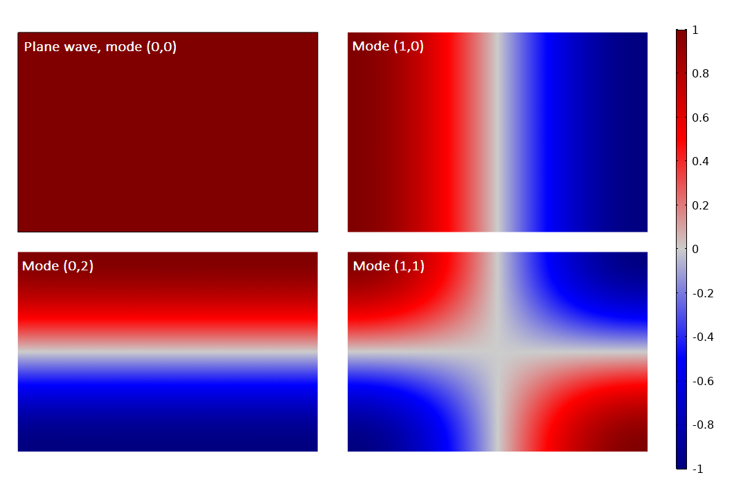
The new Port boundary condition is used to excite and absorb acoustic waves that enter or leave waveguide structures, like ducts and channels. The condition is available in the Pressure Acoustics, Frequency Domain interface. To provide the full acoustic description at a waveguide inlet/outlet, you can combine several port conditions on the same boundary. By including all relevant propagating modes in the studied frequency range, the port conditions provide a near-perfect, nonreflecting radiation condition for waveguides. In essence, this represents a multimode expansion of the solution. In many cases, using the new Port condition provides superior ease of use and accuracy compared to a plane-wave radiation condition or a perfectly matched layer (PML) configuration. The Port condition allows for automatic S-parameter (scattering parameter) calculation and has built-in postprocessing variables to easily compute the transmission loss (TL) or the insertion loss (IL). The Port condition can also be used as a source to just excite a system with a specific mode.
You can see this functionality used in the following models:
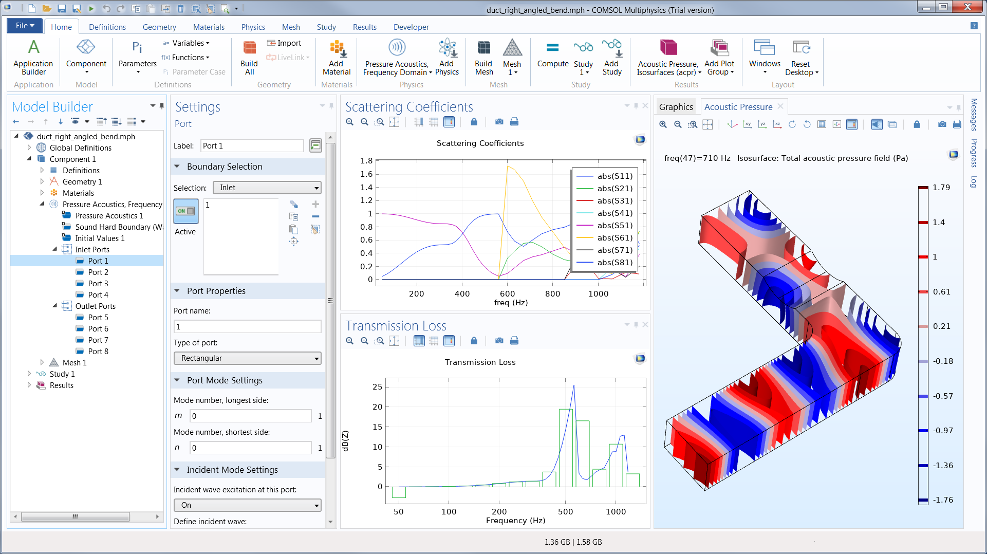
Port feature Settings window with the rectangular port type selected and wave excitation enabled for the plane wave mode (0,0). The results show the computed scattering coefficients and transmission loss of the duct system, as well as an isosurface plot of the pressure at 710 Hz.
Nonlinear Acoustics Westervelt Model
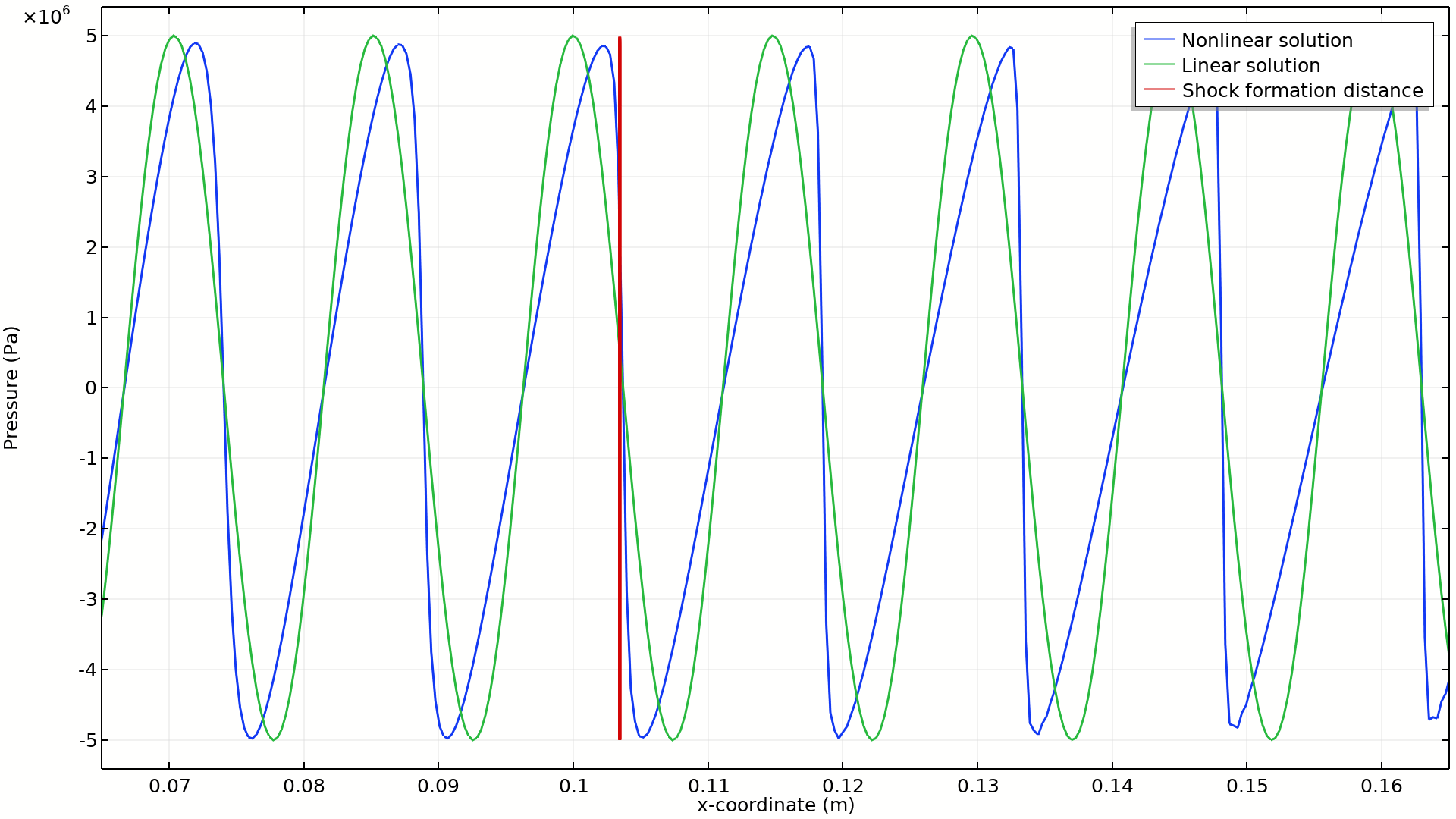
At high sound pressure levels, the propagation of pressure waves can no longer be described by the linear acoustic wave equation; solving the full nonlinear second-order wave equation is required. This equation can be simplified when cumulative nonlinear effects dominate local nonlinear effects, for example, when the propagation distance is greater than the wavelength. This is captured by the new Nonlinear Acoustics (Westervelt) feature available with the Pressure Acoustics, Time Domain interface. The feature can be used to model high amplitude acoustics in the time domain as experienced in some transducers, acoustic horns, and ultrasound uses. The new functionality also includes shock capturing stabilization and specialized solver handling.
You can see this functionality used in the following models:
Nonlinear propagation and shock formation modeled using the Nonlinear Acoustics (Westervelt) feature. The propagation after the shock formation is captured using specialized stabilization.
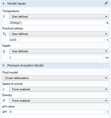
Atmosphere and Ocean Attenuation Material Models
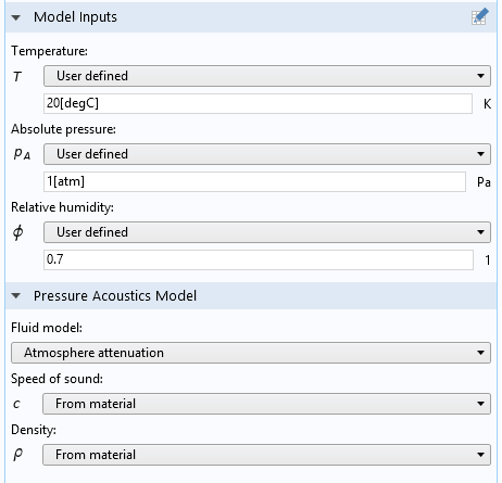
Two new material models for attenuation, one for atmospheric air and one for ocean water, are now included in the frequency domain Pressure Acoustics interfaces and the Ray Acoustics interface. Both models are semianalytical and calibrated with extensive measurement data. They include effects due to viscosity, thermal conduction, and relaxation processes of various molecules. The Atmosphere attenuation model defines attenuation that follows the ANSI standard S1.26-2014. The model depends on atmospheric pressure (absolute pressure), temperature, and relative humidity. The Ocean attenuation model depends on temperature, salinity, depth, and pH value, and for this model there is no established standard. The attenuation effects in both air and water are important for propagation over large distances and for high-frequency processes. Both models are especially important in ray tracing simulations where propagation can be simulated over very large distances. You can see this functionality used in the Underwater Ray Tracing Tutorial in a 2D Axisymmetric Geometry model.
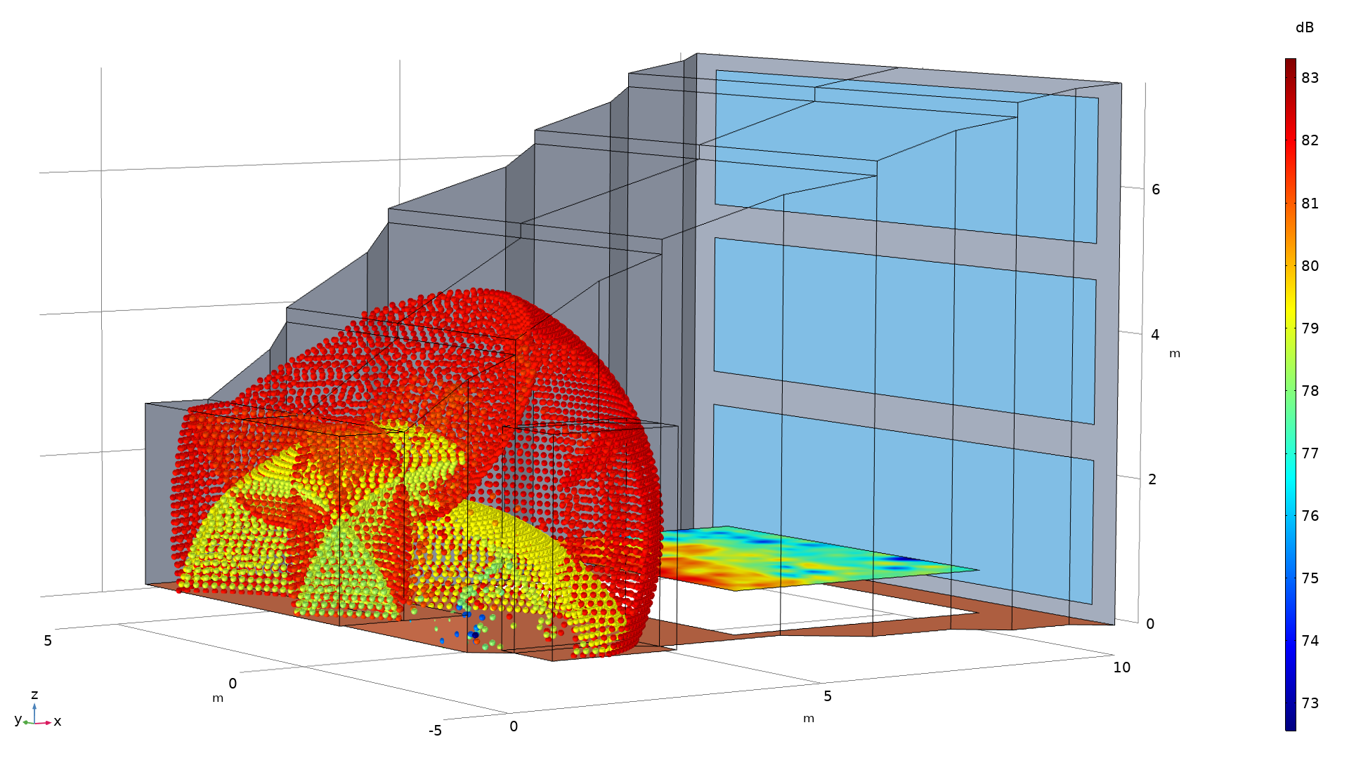
Exterior Field Calculation
The new Exterior Field Calculation feature represents an update of the previously available Far-Field Calculation feature. The Far-Field Calculation feature has allowed for computation of the radiated field, not only in the far field (distances larger than the Rayleigh radius), but at any point outside the computational domain. In fact, the typical use was not for far-field computations. The new feature is used in the same way, but the feature name and user interface have been updated with new defaults to better reflect its use. Moreover, symmetry planes can now be visualized when setting up the model and the generated default plots have been updated to use the new functionality and defaults.
You can see this updated functionality used in the following models:
- vented_loudspeaker_enclosure
- loudspeaker_driver
- lumped_loudspeaker_driver
- tonpilz_transducer
- piezoacoustic_transducer
- acoustic_scattering

The user interface for the new Exterior Field Calculation feature. In the Graphics window, the symmetry planes used for evaluation are highlighted.
Exterior Field Calculation for Pressure Acoustics, Time Domain Interfaces
The Exterior Field Calculation feature can now be used in all transient Pressure Acoustics interfaces when combined with a Time to Frequency FFT study step. The feature will only generate variables and default plots that can be used in results when time-dependent simulation data has been transformed to frequency domain data using a Time to Frequency FFT study step. You can see this functionality in the tutorial named Acoustic Horn: Nonlinear Sound Propagation Using the Westervelt Model.
Additional Boundary Element Functionality
An improved solver strategy for hybrid BEM-FEM models has been implemented, which gives a significant speedup in most models, most significantly in models with a large fraction of the FEM degrees of freedom. The functionality of the Pressure Acoustics, Boundary Element interface has been extended with functionality previously only available in the corresponding finite-element-based interface:
- Multiphysics couplings to the Thermoviscous Acoustics and Poroelastic Waves interfaces
- The Interior Velocity and Interior Displacement boundary conditions
- All of the impedance models in the Impedance condition (for example RCL circuit, Physiological, etc.)
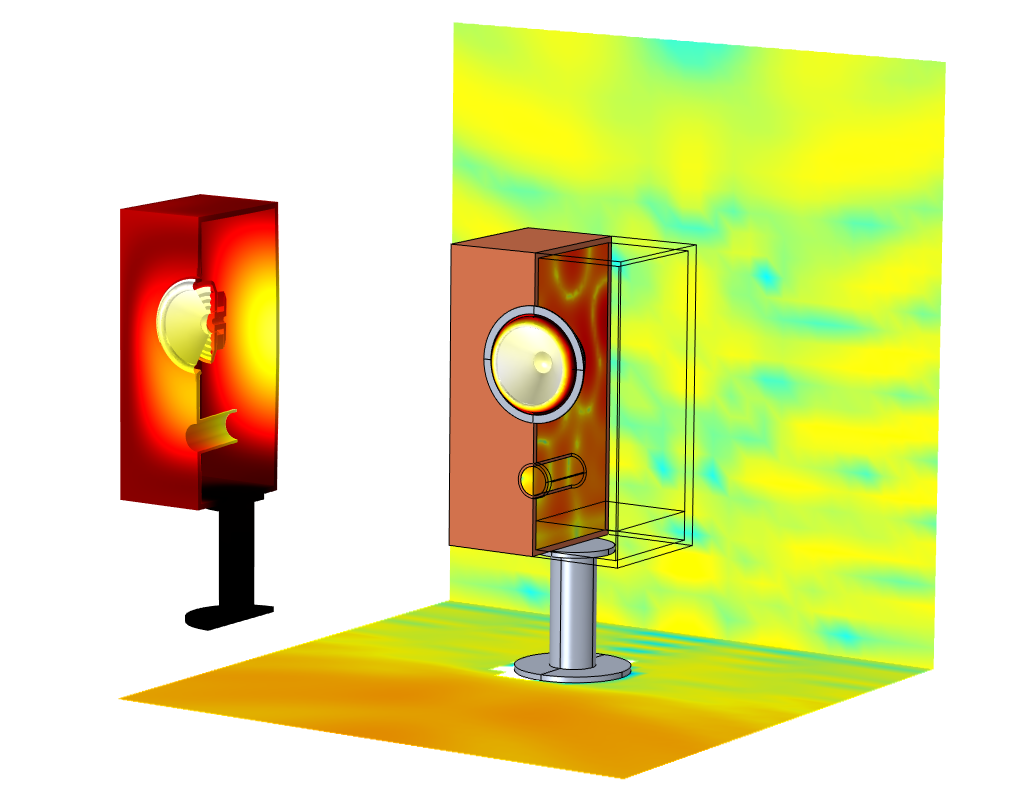 The new solver strategy for hybrid BEM-FEM models shows a great speedup on the Vibroacoustic Loudspeaker Simulation: Multiphysics with BEM-FEM model. On a particular hardware configuration, the solution time decreases from 1h 37 min to 51 min.
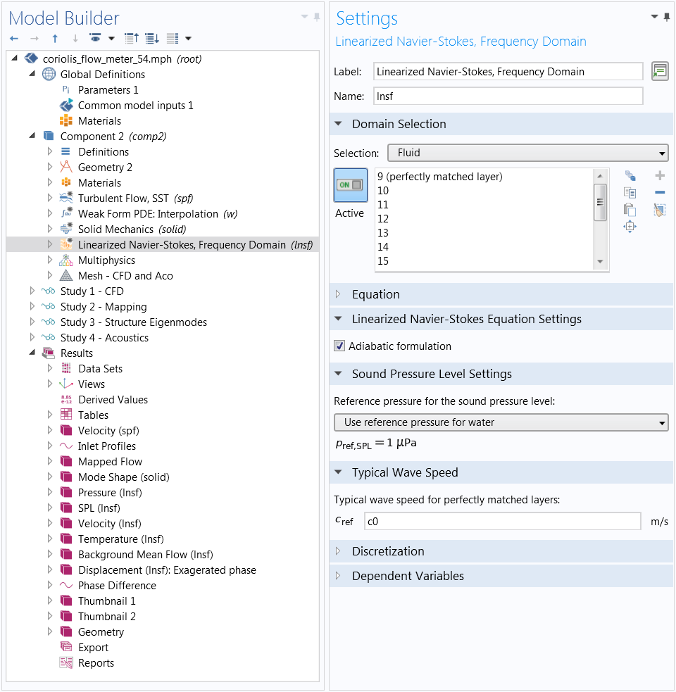
Adiabatic Formulation Option for Linearized Navier-Stokes and Thermoviscous Acoustics
The Linearized Navier-Stokes and Thermoviscous Acoustics physics interfaces now have an option to use an Adiabatic formulation for the governing equations. This formulation is a good approximation for most liquids, like water, where the thermal effects are small compared to the viscous effects. An added benefit of using the new option, when physically valid, is that it reduces the computational cost of the model. This is because the temperature degree of freedom (DOF) is no longer solved for, but is directly related to the pressure (adiabatic).
The following models use this feature:
Gradient Term Suppression (GTS) Stabilization for Linearized Navier-Stokes
The linearized Navier-Stokes physics interfaces now have the option to use Gradient Term Suppression Stabilization. When the linearized Navier-Stokes equations are solved, linear physical instability waves can develop, known as Kelvin-Helmholtz instabilities. These instabilities can grow over time or when solving the system with iterative solvers. The terms responsible for the instabilities are typically the reactive terms in the governing equations. In some problems, the growth of these instabilities can be limited, while the acoustic solution is retained, by canceling terms involving gradients of the mean-flow quantities. This is what is known as gradient term suppression stabilization. The terms that can be excluded are grouped into Reactive terms and Convective terms.
New and Updated Default Plots
There are multiple updates to the default plots. The color schemes are now consistent across physics interfaces. For example, the Wave color table has a symmetric range to represent the acoustic pressure and the ThermalEquidistant color table represents the acoustic temperature variations in thermoviscous acoustics. When performing an eigenfrequency analysis, a new Evaluation Group is added by default with information about the eigenfrequency, damping ratio, and quality factor. Default plots of the exterior field have been updated to use new functionality and defaults.
You can see this new functionality in the following models:
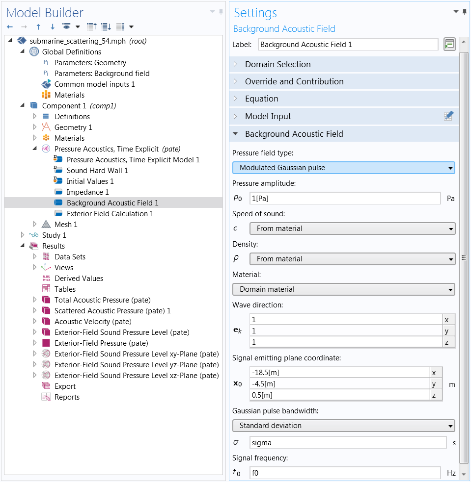
Modulated Gaussian Pulse Option for Background and Incident Fields
The transient Pressure Acoustics interfaces have a new option to define a Modulated Gaussian pulse as a background acoustic field or as an incident acoustic field. The option is useful when modeling scattering problems in the time domain, for example. In such cases, the modulated Gaussian pulse can be tuned to have a band-limited frequency content centered on a carrier frequency.
Animation of the propagation and scattering of a Gaussian pulse by a submarine, visualized as isosurfaces.
Air and Water Materials Updated with Acoustics-Specific Quantities
The Air and the Water, liquid materials in the Built-In Materials section have been updated to include material data that can be used to simplify the modeling of acoustics problems. For both materials, the value of the bulk viscosity has been added, as well as the coefficient of thermal expansion. For water, a temperature-dependent expression for the ratio of specific heats has also been added. To take advantage of the new and updated material data, when opening an existing model, delete the material and add it again from the Add Material window.
This functionality is used in the following models:
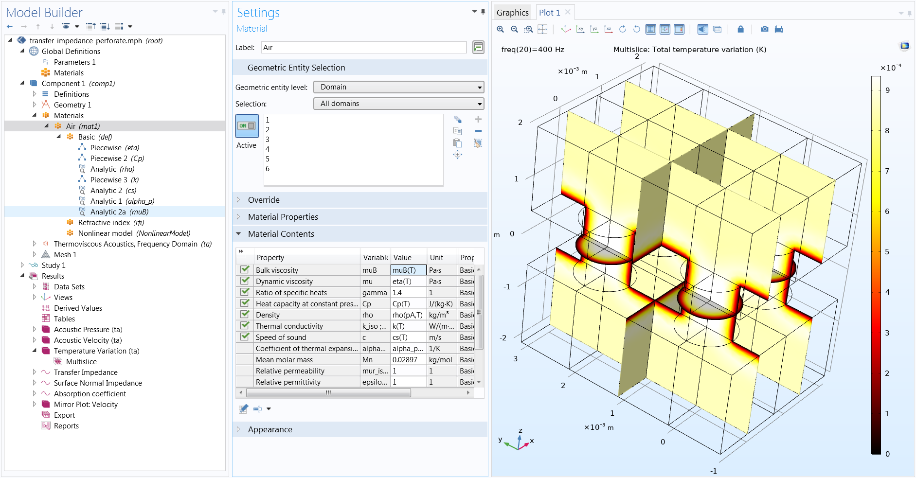
Models that use the Thermoviscous Acoustics or the Linearized Navier-Stokes physics interfaces take advantage of the addition of the Bulk viscosity to the Air material.
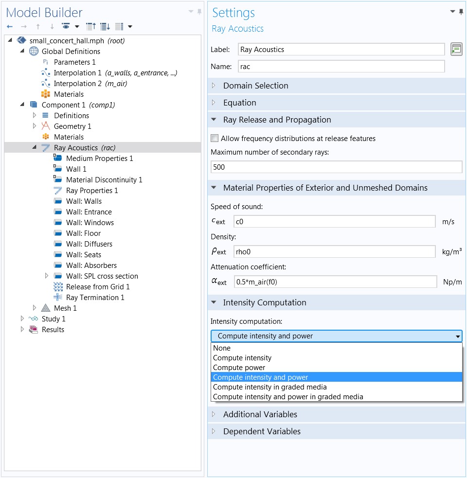
Ray Acoustics Updates
The Ray Acoustics interface has an improved method for calculating intensity in absorbing and attenuating media, making it possible to include domain attenuation in unmeshed ray tracing models as well as in the void domain outside the geometry. The overall accuracy of the intensity computation has also been improved. A new section called Material Properties of Exterior and Unmeshed Domains has been introduced with an input field for the attenuation coefficient, along with the speed of sound and the density inputs. On Wall conditions, the behavior for the Rayleigh roughness model has been improved for consistency. The Ray Acoustics interface also has a new option for intensity computation, Compute power, which uses fewer DOFs than the option Compute intensity and power, while still being able to compute the sound pressure level on boundaries and plot the impulse response. However, to plot the intensity or sound pressure level along rays, you must still select Compute intensity or Compute intensity and power.
This new functionality is used in the following models:
Important Enhancements and Bug Fixes
General Enhancements
- The underlying geometry is now visible when performing a preview plot of a grid dataset, and the geometry is shown for preview plots of cut points, cut lines, and cut planes that refer to a grid dataset
- Polar plots now have improved control of the axis orientation and range
- The spatial frame is now always used when evaluating outside meshed domains with the Radiation Pattern plot, Grid datasets, or Parameterized Curve/Surface datasets
- The Ideal gas option for density representation is available in the Linearized Navier-Stokes interfaces
- The From speed of sound option to define both compressibility and thermal expansion is available in the Linearized Navier-Stokes and Thermoviscous Acoustics interfaces
- The stabilization for the Linearized Navier-Stokes interfaces has been improved in situations where the background flow has large gradients
- In most of the physics interfaces, the Periodic Condition now has a user-defined option to control which field components are coupled
Postprocessing Enhancements
- Impedance variables are now defined on prescribed acceleration, velocity, and displacement boundaries in the Pressure Acoustics, Frequency Domain interface
- A predefined variable now exists for the lumped characteristic impedance in the Thermoviscous, Boundary Mode interface
- On impedance boundary conditions, postprocessing variables are defined for the normal incidence absorption (
acpr.imp1.alpha\_n) and the random incidence absorption (acpr.imp1.alpha\_ran)
Solver Enhancements
- The iterative solver suggestion now works for eigenfrequency problems with Thermoviscous Acoustics
- The Aggregation option is now used for all solver suggestions that are based on the domain decomposition preconditioner; this method is fully parallelized
- An iterative solver suggestion is now generated when using the Solid-Shell multiphysics coupling and pressure acoustics, in both the FEM- and BEM-based interfaces
New and Updated Tutorial Models and Applications
COMSOL Multiphysics® version 5.4 brings several new and updated tutorial models and applications.
Duct with a Right-Angled Bend
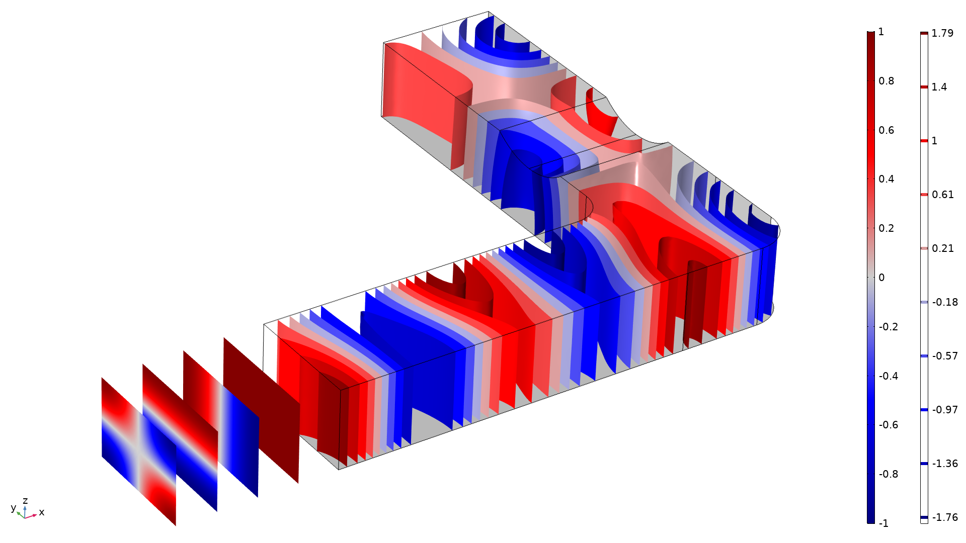
Acoustics of a waveguide with a right-angled bend analyzed using the new Port boundary condition. In this figure, the modes used at the inlet are depicted away from the geometry.
Search in the Application Library:
duct_right_angled_bend
Small Concert Hall Acoustics
This ray acoustics tutorial is now part of the Application Library and includes detailed step-by-step instructions, using the new attenuation computation available for unmeshed domains.
Search in the Application Library:
small_concert_hall
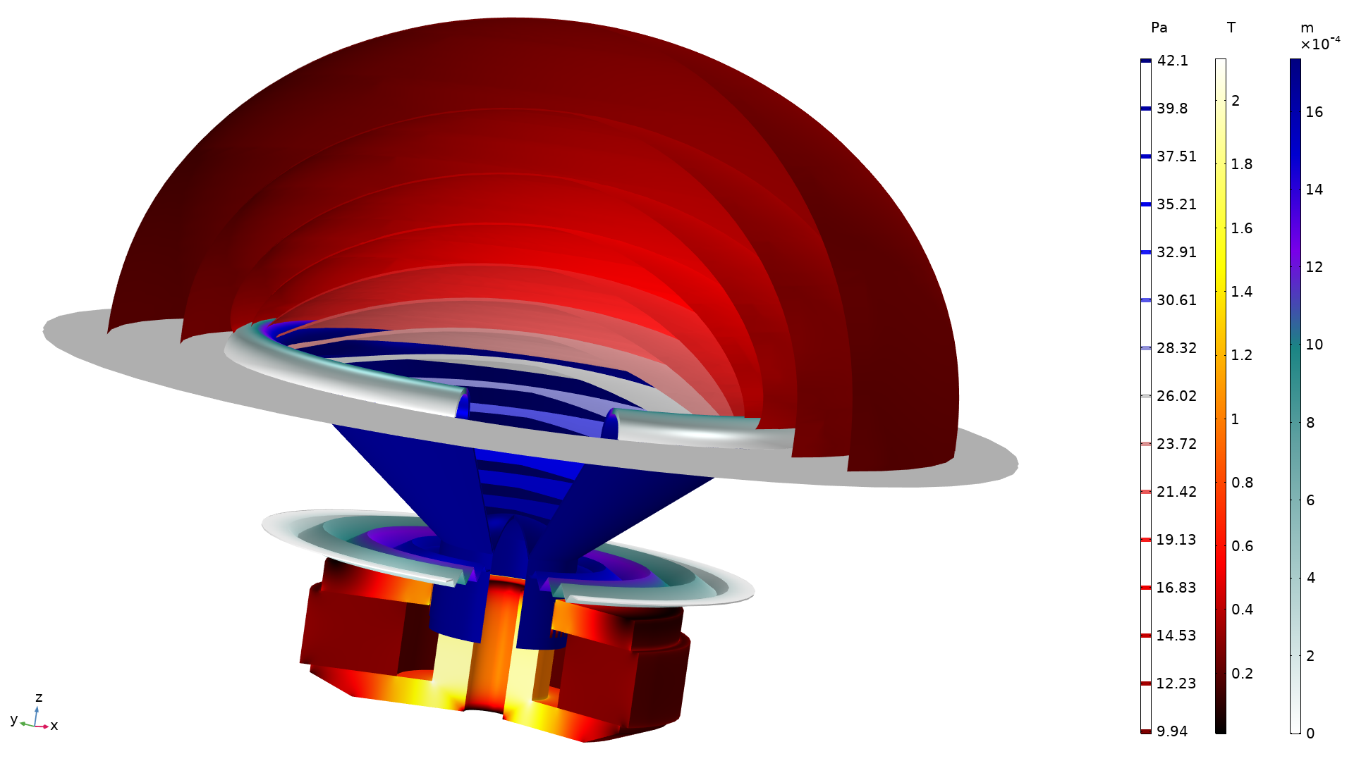
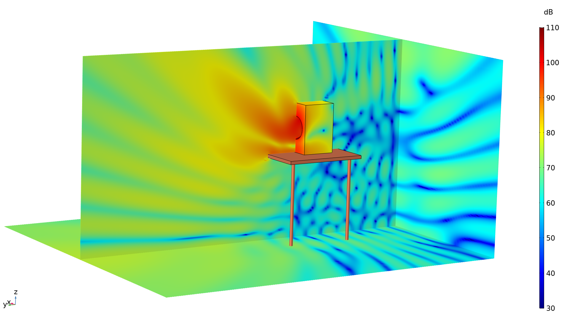
Lumped Receiver with Full Vibroacoustic Coupling
 Full vibroacoustic analysis of the interaction between a vibration isolation mounting and a miniature hearing aid transducer. Shown here: The deformation of the ear-mold tube and receiver and the sound pressure level in the coupler volume.
Search in the Application Library:
lumped_receiver_vibroacoustic
Loudspeaker Driver, Transient
 Full transient multiphysics analysis of a loudspeaker driver, which allows the modeling of nonlinear effects. The results include the total harmonic distortion (THD) and the dynamic BL curve.
Search in the Application Library:
loudspeaker_driver_transient
Nonlinear Acoustics — Modeling of the 1D Westervelt Equation
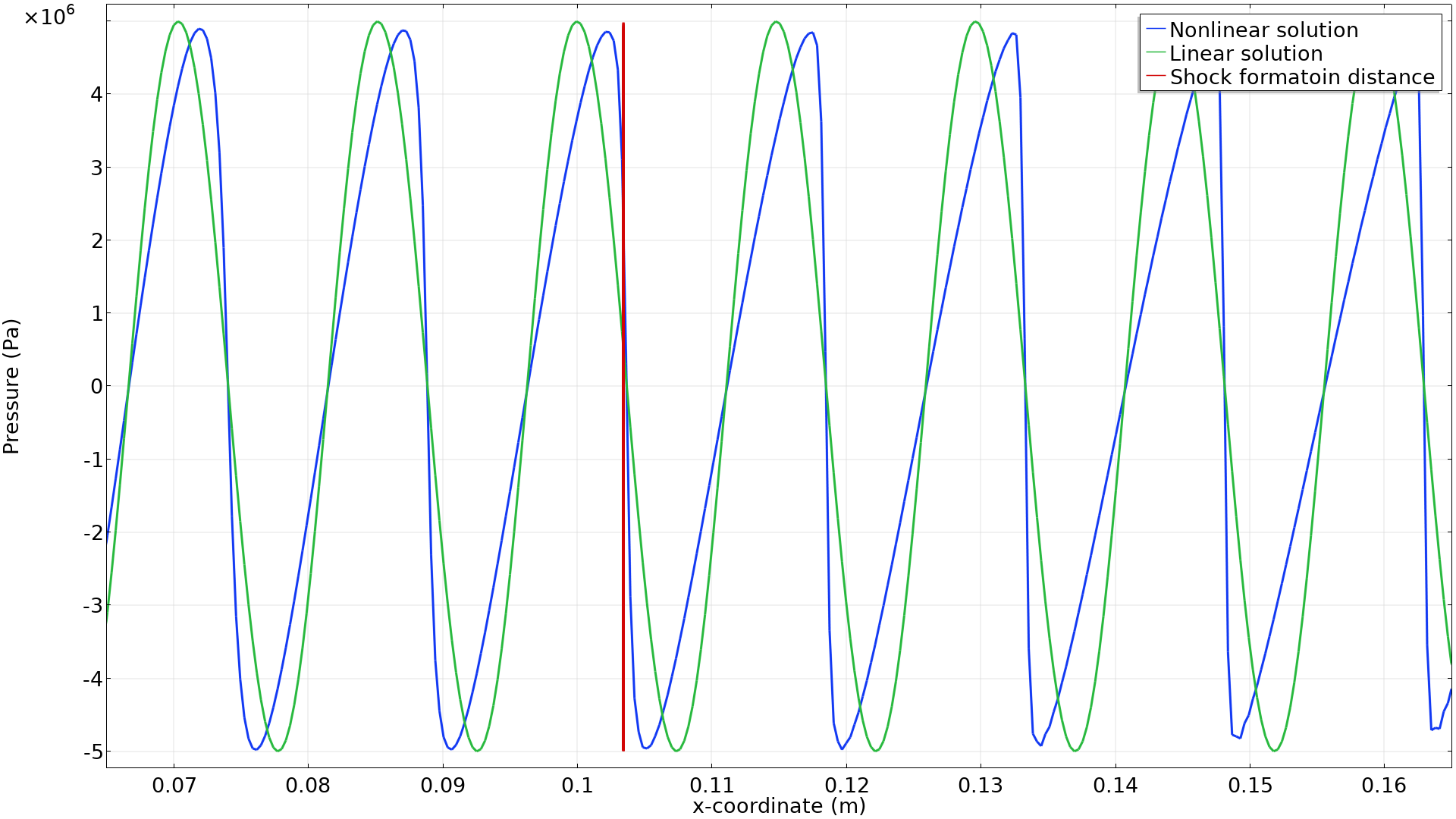 Transient nonlinear propagation of finite-amplitude acoustic waves in a fluid, by solving for the Westervelt equation. The linear and nonlinear wave profiles before and after the shock formation distance are shown.
Search in the Application Library:
nonlinear_acoustics_westervelt_1d
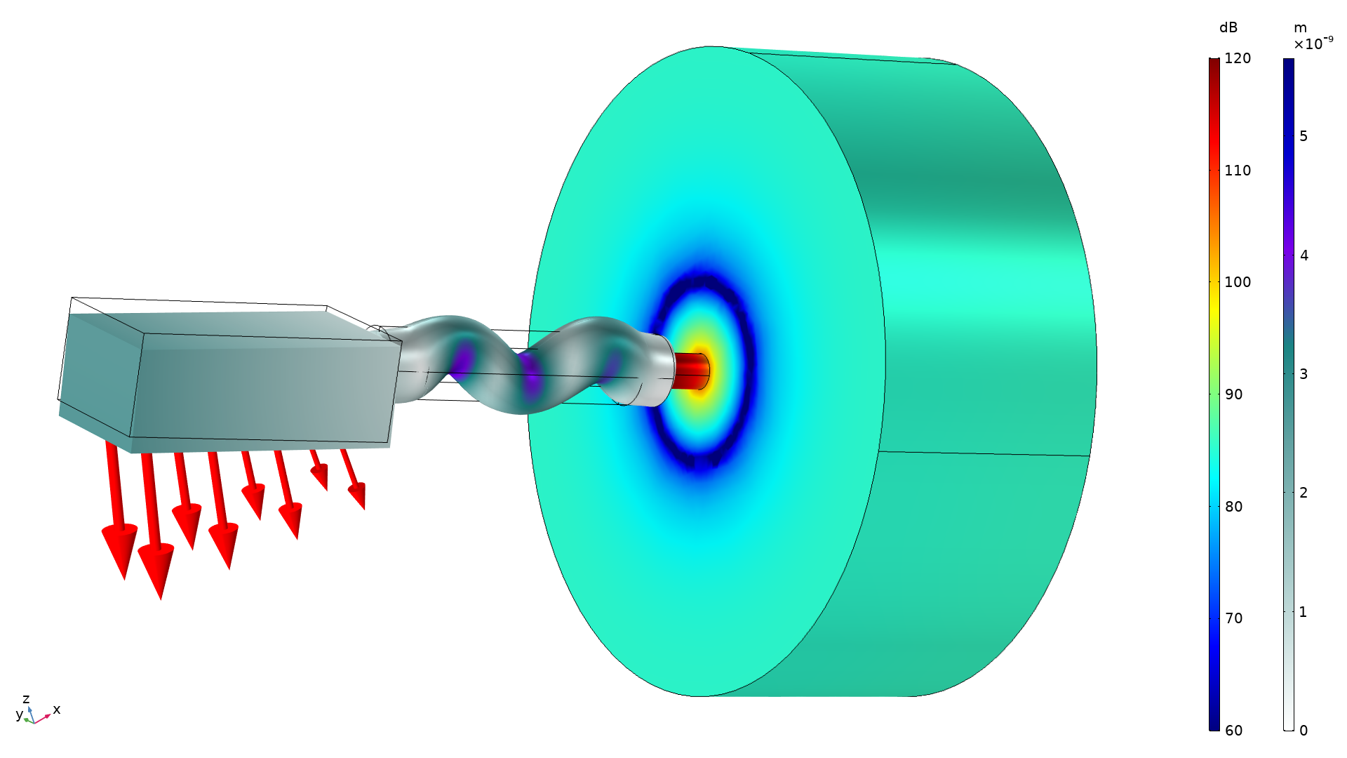
Radiation from a Baffled Piston

An axisymmetric model of a rigid piston in an infinite baffle is used to exemplify the Exterior Field Calculation feature; the image shows the pressure field evaluated in a cross-section plane.
Loudspeaker Radiation: BEM Acoustics Tutorial
 Acoustic radiation pattern from a small loudspeaker analyzed using the boundary element method. The sound pressure level radiated from the loudspeaker at 2000 Hz is shown.
Acoustic Horn: Nonlinear Sound Propagation Using the Westervelt Model
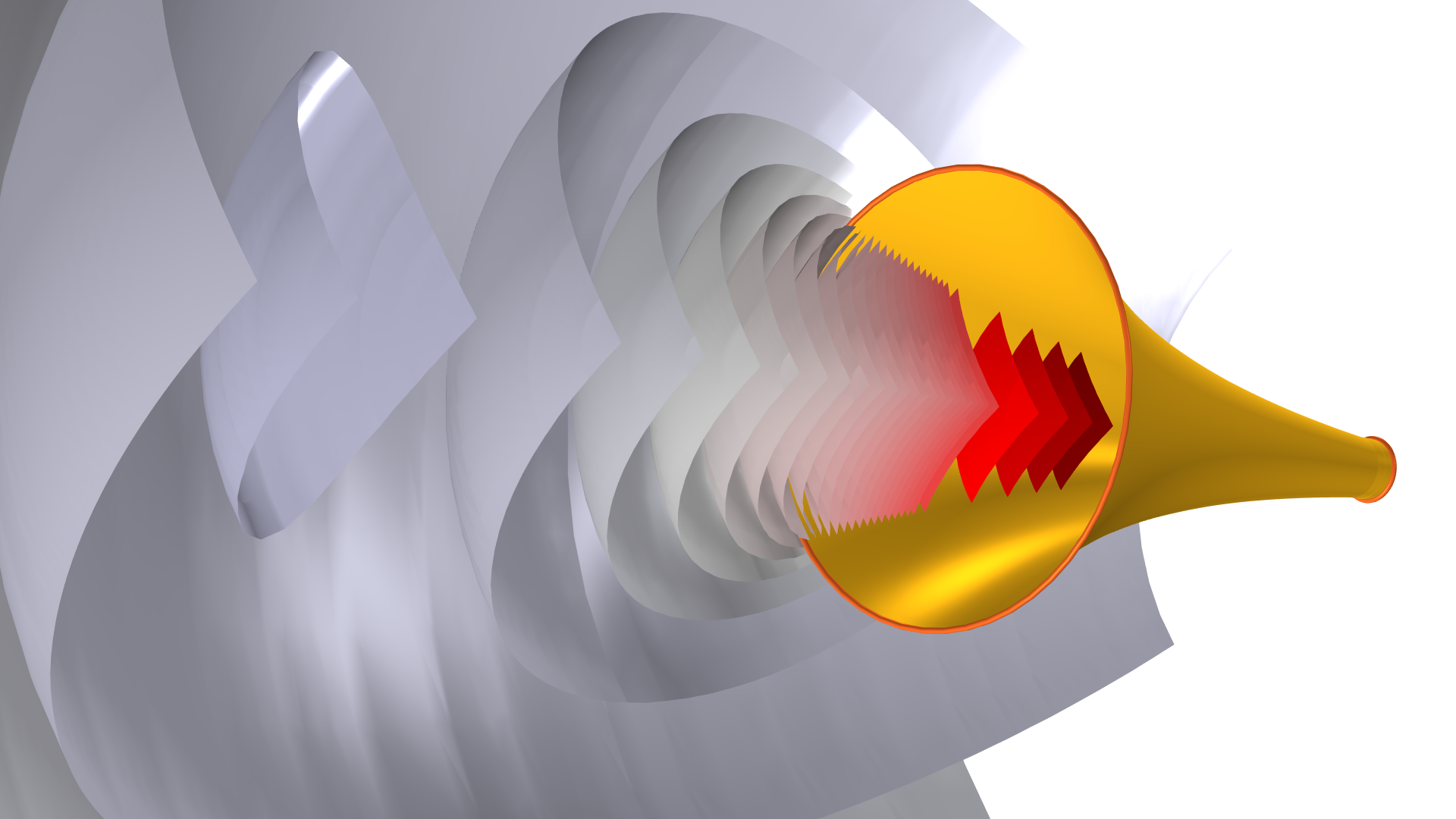 This tutorial shows how to include local nonlinear effects when simulating the acoustics of an exponential horn. Nonlinear effects become important when an acoustic horn is used for high-amplitude signaling.
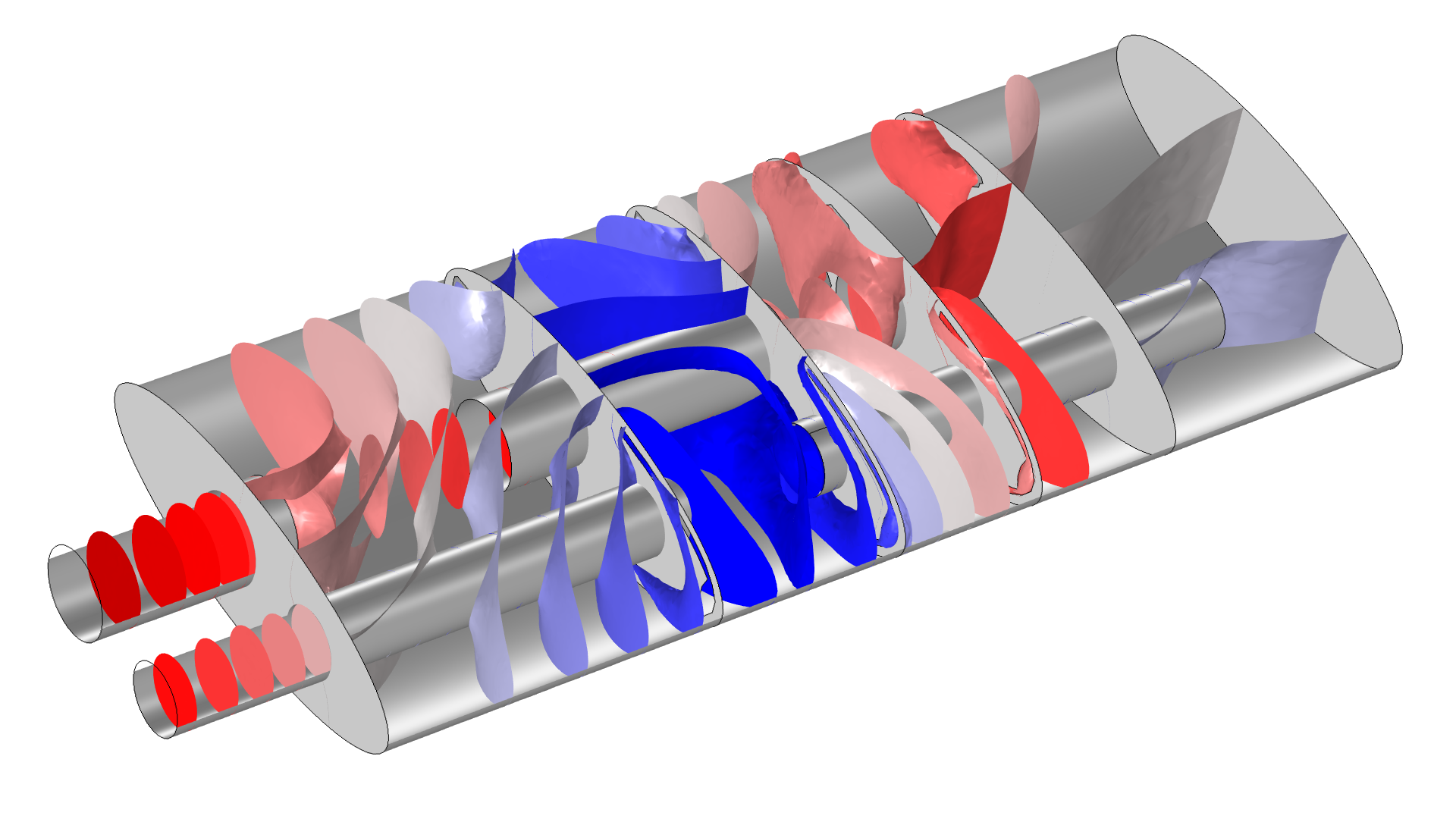
Sonic Well Logging
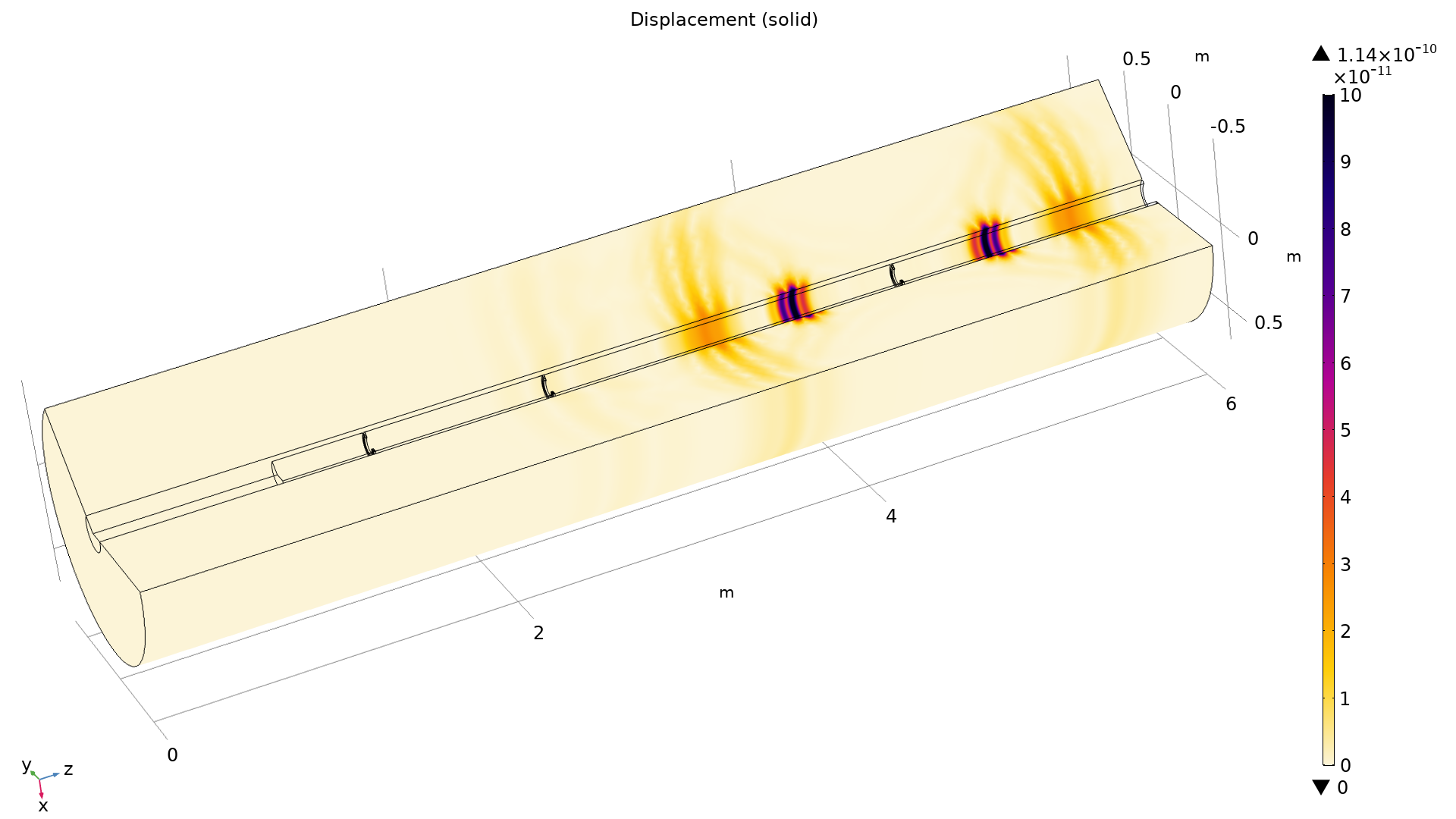 This model demonstrates how to simulate a piezoelectric transducer both as a sound transmitter and a receiver in a well logging setup. Here, the displacement field of the elastic wave is shown.
Muffler with Perforates
This tutorial model has been updated to use the new Port boundary conditions, simplifying the model setup and postprocessing of the transmission loss.
Search in the Application Library:
perforated_muffler
Helmholtz Resonator with Flow

The CFD part of this tutorial has been updated to use the new Fully developed flow option of the Inlet boundary condition, now available for the SST turbulence model.
Search in the Application Library:
helmholtz_resonator_with_flow