Study and Solver Updates
COMSOL Multiphysics® version 5.4 includes faster solving with newer processors in Windows® thanks to new memory allocation, up to 15% faster CFD simulations due to new reusing of sparsity pattern, Parametric Sweeps over parameter groups, and optimization for Parametric Sweeps. Learn more about all of the updates relating to studies and solvers below.
Several Times Faster Solving in the Windows® Operating System
Thanks to a new and more efficient method for memory allocation, the overall solver performance has improved by several times for certain processor architectures in the Windows® operating system. The performance improvement is only seen for recent processor architectures when using eight or more cores. For macOS and the Linux® operating system, this level of performance has been available since earlier versions.
Up to 15% Faster Simulations
Earlier versions of COMSOL Multiphysics® included performance improvements based on reusing data from previous matrix assembly and solver steps. Continuing this development into the latest version, new solver functionality reuses the system matrix sparsity pattern from a previous step, which is important for nonlinear and time-dependent analyses. The functionality takes a little more memory, typically a few percent more, but can give up to 15% reduction in solution time. By default, the new Reuse sparsity pattern option is enabled for many of the physics interfaces used for fluid flow, transport phenomena, and structural mechanics. For other physics, the Reuse sparsity pattern option is disabled by default, but it can be manually enabled under the Advanced solver node and its Assembly Settings section.
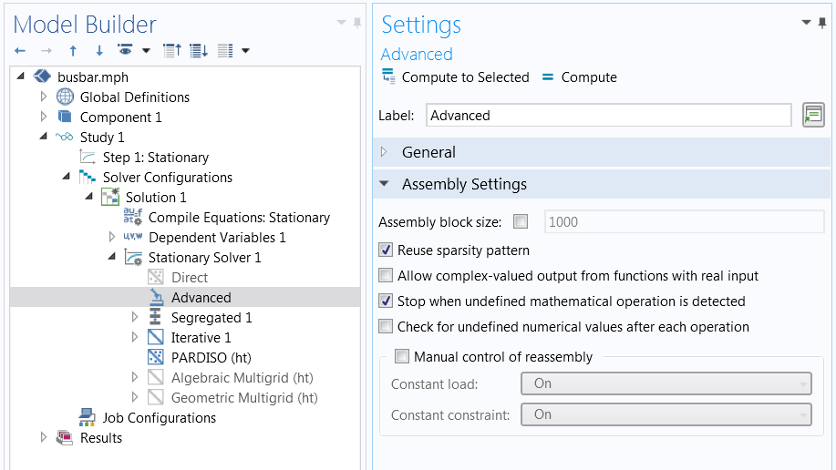
The solver setting to enable/disable the Reuse sparsity pattern option.
Parametric Sweeps Over Parameter Cases
With COMSOL Multiphysics® version 5.4, you can structure your parameters by creating multiple Parameters nodes. Furthermore, Parameters nodes support Cases, which let you switch between different sets of parameter values without importing and exporting them to file. For the Parametric Sweep functionality, there is a new option called Parameter Switch for sweeping over different parameter Cases.
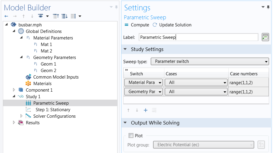
Two Parameter groups for materials and geometry, with two sets of values each; the Parametric Sweep can be used to solve for all four combinations of Cases.
Optimization for Parametric Sweeps
You can now optimize over a general Parametric Sweep study including sweeps over geometric dimensions. This functionality is useful when several sets of fixed parameter values need to be considered in an optimization problem alongside one or more control parameters. Note that this functionality is different from what is known as discrete optimization.
The objective function is interpreted as either a sum, maximum, or minimum over the Parametric Sweep study solutions. The new Optimization setting controlling the objective definition is called Outer solution. In this context, an outer solution is a parametric sweep solution over a parameter such as a geometric dimension. In contrast, an inner solution is, in the Optimization settings, referred to as just Solution. An inner solution is coming from a Time-Dependent, Eigenfrequency, or Auxiliary Sweep study. Optimization has been supported for inner solutions in previous software versions.
For inner solutions (with the exception of eigenfrequency solutions), gradient-based optimization methods can be used. The new functionality that also covers parametric sweeps can only be used with the gradient-free optimization methods. It is now also possible to run a Parametric Sweep study with an Optimization study; this functionality can be used to solve one optimization problem for each outer parameter.
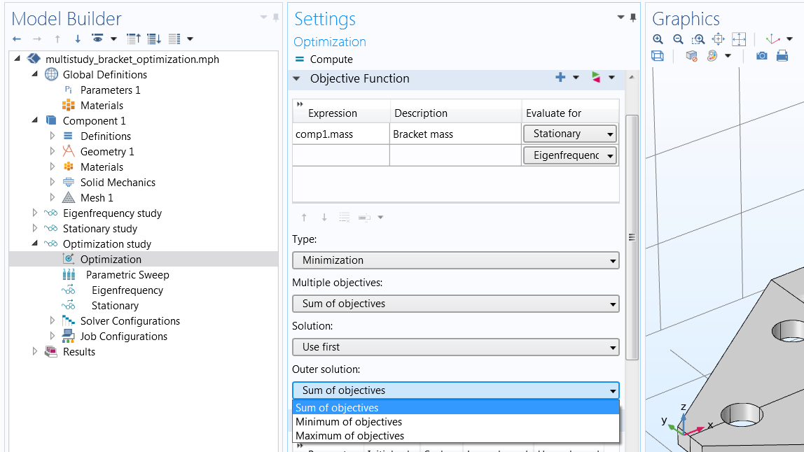
Combine Optimization and Parametric Sweeps with the new setting for Outer solution for the Optimization study.
Adaptive Mesh Refinement Solution Container
When solving with adaptive meshing, the adaptation method now stores the solutions in a container node similar to the functionality of a parametric sweep. A mesh refinement level parameter is automatically added, which makes results comparisons easier, as all the solutions can be obtained from one dataset.
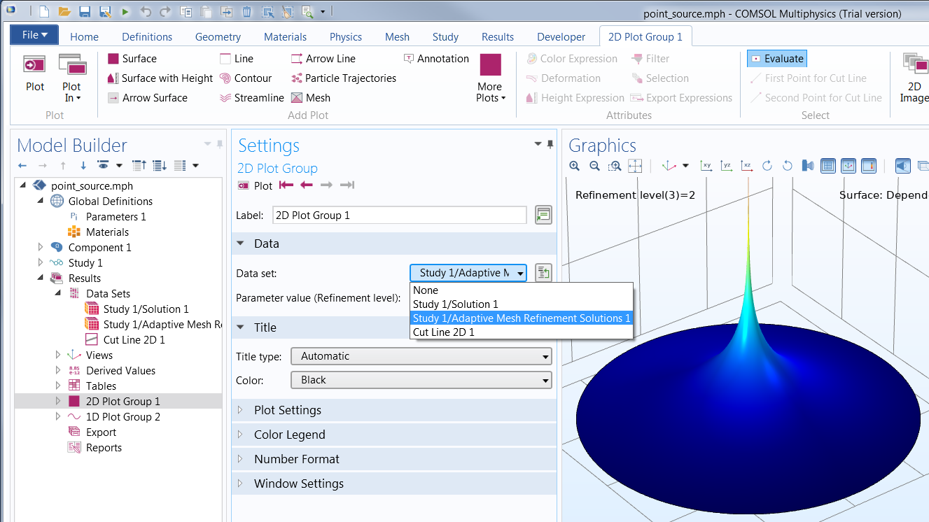
Using the new Adaptive Mesh Refinement dataset for the automatically mesh-refined solutions, shown here for the Point Source model.
Reduced Model Inputs Moved to Definitions
The Model Inputs declaration for reduced-order models has been moved from the Model Reduction study to the Global Definitions node. You can now define the expressions for reduced-order model variables in one place. These expressions will be used for both the reduced and unreduced versions of the model. When the reduced model is built by the Model Reduction study, the training expression value will be used. This training value is still specified at the study level.
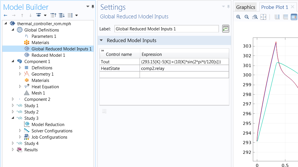
The specification of two Global Reduced Model Inputs and their expressions for the thermal_controller_rom model. The training expressions for the Reduced Model Inputs are still specified in the Model Reduction study.
New TFQMR Iterative Linear Solver
A new iterative method for linear equations has been added: TFQMR. This is a transpose-free version of the quasi-minimal residual (QMR) method. The QMR family of methods only stores a fixed number of solution vectors, independent of the number of iterations, and the residual is minimized in a quasi sense. QMR will therefore behave similarly to GMRES but without the cost of restart vectors. The downside of the method is that it needs more iterations to converge (for the same matrix and the same preconditioner). Each iteration with QMR is less expensive than for GMRES, so it is not possible to say beforehand which method is fastest for a specific matrix. However, QMR will use less memory than GMRES, especially for cases where the GMRES restart number (default 50) needs to be increased in order to reach convergence. Computations falling in this category include those where multigrid or other high-quality preconditioners cannot be used.
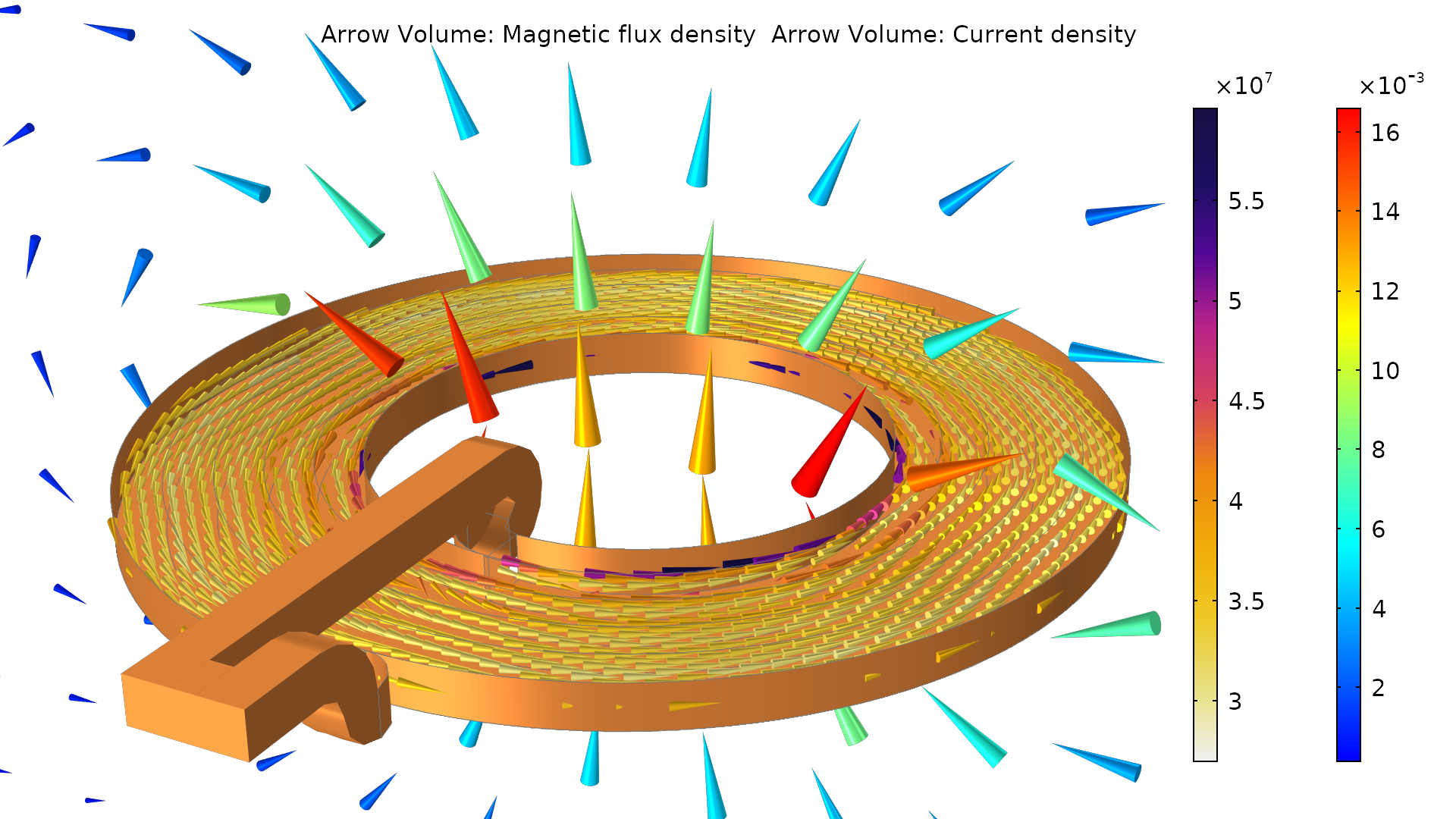 For the Spiral Coil with Epoxy Varnish Insulation model, the new TFQMR solver preconditioned with SSOR is used to solve a linear element version of this model with 901k DOFs. The computation needs 2.8 GB memory and takes 656 seconds, as compared to 13.4 GB and 1242 seconds for GMRES.
Modified Default Factor in Error Estimate for Direct Linear Solvers
The default for the Factor in error estimate setting that is applied to the direct solvers has been changed. The new default is 1, as compared to 400 previously. This change applies only to a direct solver when it is used as the main solver and not when it is used as part of a preconditioner, where 1 is the default already. Note that this change promotes easier error testing by making the linear solver error estimate 400 times smaller. Using this new default typically makes the error estimate more accurate and avoids unnecessary iterative refinement and warnings/errors.
More Robust Automatic Newton Solvers for Automatically Scaled Variables
For some nonlinear simulations, the scales of the dependent variables are difficult to find for the automatic scaling method, and they can also dramatically change during nonlinear iterations. For automatically scaled dependent variables, a new method now updates the weights used for measuring the errors in the automatically damped Newton methods. When the weights are updated, the Newton solver is restarted. This makes the automatic Newton solvers more robust, and can lead to fewer overall iterations. However, there is also a risk that the restart of the solver will cost some extra iterations compared to not performing a restart. For this reason, the new method is not enabled by default. The new method is enabled by setting Update weights for automatic scales to Use threshold for weights, and it is available from the Method and Termination section for the Fully Coupled and Segregated Step nodes under the Stationary solver.
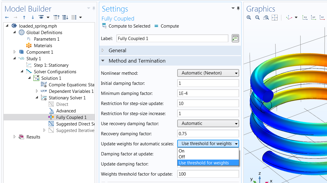
Settings for the Use threshold for weights for the automatically damped Newton methods.
Linux is a registered trademark of Linus Torvalds in the U.S. and other countries. macOS is a trademark of Apple Inc., in the U.S. and other countries. Microsoft and Windows are either registered trademarks or trademarks of Microsoft Corporation in the United States and/or other countries.