Geometry and Mesh Setup for Modeling Regions of Infinite Extent
For many cases, it is important to be able to represent an unbounded region. COMSOL Multiphysics® contains features and functionality that enable you to model a region of infinite extent. This article explains the different options available for modeling such a region and the application areas for which they are used. We will also address the modeling setup and meshing of these regions.
Functionality for Modeling Domains of Infinite Extent
There are four options for modeling a region of infinite extent and they each have different areas of applicability:
- The Infinite Element domain functionality is meant for governing equations that are diffusion-like in nature. Interfaces where it is commonly used include Heat Transfer in Solids, Electrostatics, Electric Currents, and Magnetic Fields. Infinite elements represent a region that is stretched along certain coordinate axes with the effect of approximating an infinitely large domain.
- The Perfectly Matched Layer (PML) domain functionality is meant for stationary governing equations that are wave-like in nature, wherein the fields describe a radiation of energy, such as the Electromagnetic Waves, Frequency Domain and Pressure Acoustics interfaces. The PML acts as a domain that is a nearly ideal absorber of radiation.
- The Absorbing Layer functionality is the time-domain analogue of the PML. It is also meant for governing equations that are wave-like in nature but are solved via a time-explicit approach, such as in the Electromagnetic Waves, Time Explicit and Pressure Acoustics, Time Explicit interfaces.
- The Hybrid BEM-FEM approach is available for certain combinations of physics. This uses a finite element formulation within the modeled volume, and a boundary element formulation over the exterior surfaces. The hybrid BEM-FEM approach is exemplified by the following models:
The first three options, the Infinite Element, PML, and Absorbing Layer, have specific geometry setup and meshing requirements, addressed here.
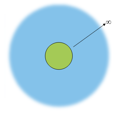
Schematic of a situation where a region of interest (green) is within a region of infinite extent (blue).
The most typical usage of these features is to model the case of a region of interest that is fully encapsulated within a region of infinite extent, as described in the image above. To accurately capture the behavior in the region of interest, one must solve the relevant governing equations in that region, as well as the region of infinite extent. However, solving for the fields in an infinitely large region is computationally impossible, so various strategies are used to truncate the model to a reasonable size. Infinite elements, PMLs, and absorbing layers are such truncation strategies that share similar setup, usage, and (with the exception of Absorbing Layers) similar meshing requirements. We will detail the geometry and meshing requirements for these three features later on in this article.
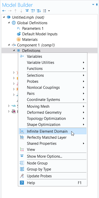
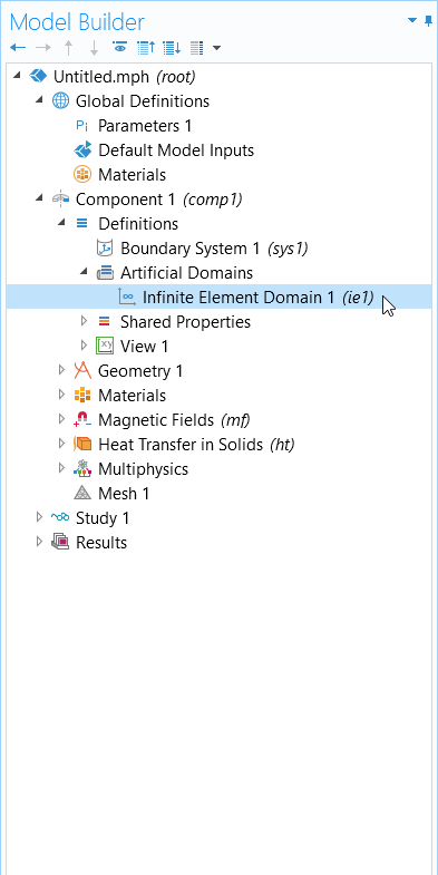
To determine if the physics you are using supports any of the above options, first add the physics to your model, and then right-click on the Definitions node or go to the Definitions toolbar. Depending upon which physics are present in your model, one, some, or none of the above options will be present.
Geometry Setup of Infinite Elements, Perfectly Matched Layers, and Absorbing Layers
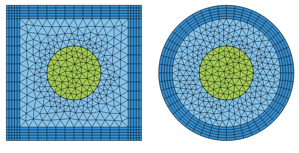
Regardless of whether infinite elements, PMLs, or absorbing layers are being used, the geometry setup is the same. If modeling in 2D, then the geometry should be set up as one of the two cases shown below, describing a Cartesian or cylindrical infinite domain.
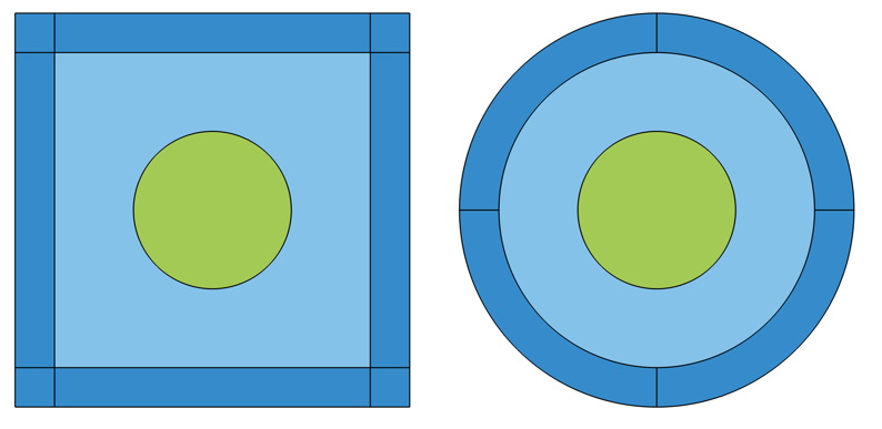
Visualization of geometry of the Cartesian (left) and cylindrical (right) infinite domains in 2D.
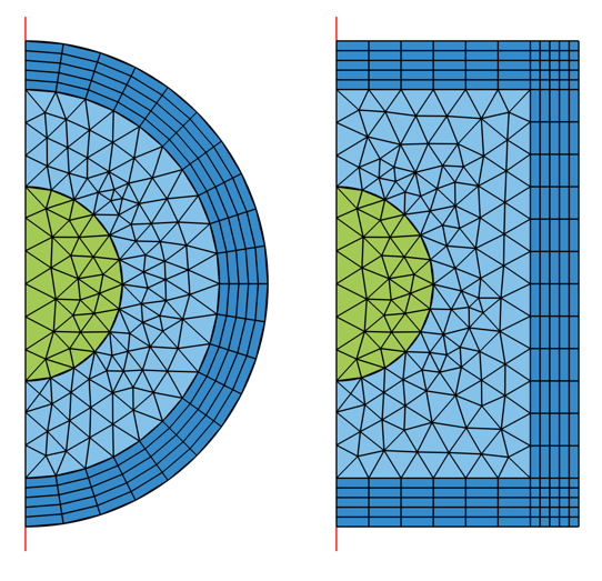
If modeling in 2D axisymmetry, the geometry should be set up as one of these two cases, describing a spherical or cylindrical infinite domain:
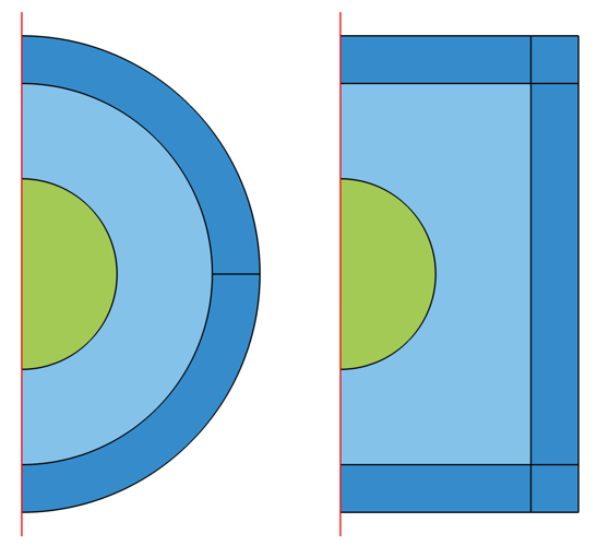
Visualization of geometry of the spherical (left) and cylindrical (right) infinite domains in 2D axisymmetry.
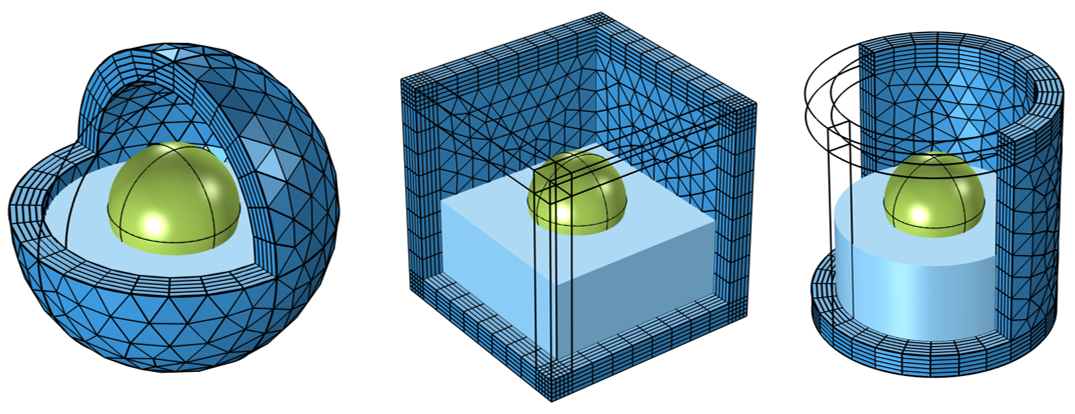
If modeling in 3D, the geometry should be set up as one of these three cases, representing a spherical, Cartesian, or cylindrical domain:
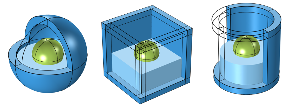
Visualization of geometry of the spherical (left), Cartesian (middle), and cylindrical (right) infinite domains in 3D. Some of the infinite domains, and the interior domain of interest, are omitted for visualization.
Note that in 2D, the Rectangle and Circle, and in 3D, the Sphere, Block, and Cylinder geometry features all include the option to introduce Layers, which will simplify the setup of the above cases. It is typical to make the thickness of these domains about one-tenth of the overall dimensions of the modeling space. The distance from the region of interest to the infinite domain is a parameter that does need to be studied. It is important that there are separate corner domains for the Cartesian and cylindrical cases.
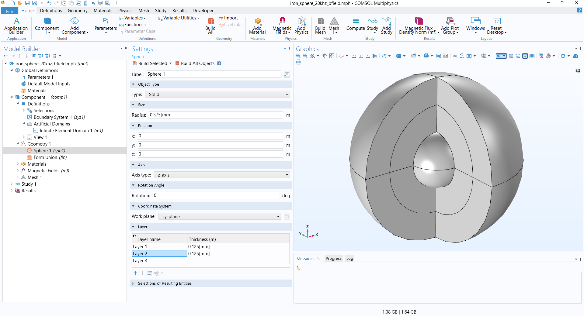 A view of the Model Builder with the model tree on the left, Settings window for the Sphere geometry in the center, and gray spherical model geometry in the Graphics window on the right.
Two layers are introduced through the Settings window of a Sphere geometry operation, under the Layers section. The Infinite Element Domain feature is assigned to the outermost layer in this model.
Special Considerations for Cylindrical and Spherical Cases
When the geometry is either cylindrical or spherical, in the 3D case, the Infinite Element, Perfectly Matched Layer, or Absorbing Layer feature will all offer the option to define a center coordinate and (for the cylindrical case) the center axis direction.
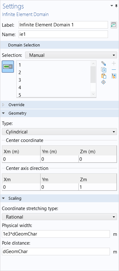
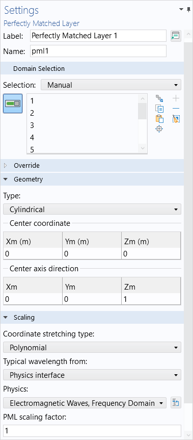
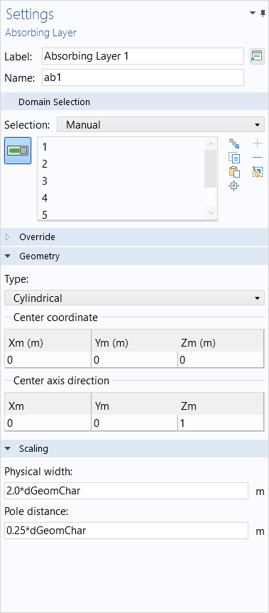
These should be adjusted based upon where and how the geometry is oriented. Although not necessary, it is often good practice to center the model about the origin and z-axis. Similarly, in 2D and 2D axisymmetry, make sure that the geometry orientation matches the feature settings.
Meshing Considerations
For the cases of infinite elements and perfectly matched layers, it is important that the mesh match the coordinate stretching direction, the direction of absorption. The meshes should look similar to what is pictured below. Use mapped meshes in 2D, and swept meshes in 3D, to produce these types of meshes. For numerical reasons, it is good for the elements in these domains to not be too distorted or stretched. We recommend starting with at least five elements through these domains and then always performing a mesh refinement study.
Visualization of appropriate Infinite Element or Perfectly Matched Layer meshes for the 2D Cartesian (left) and Cylindrical (right) cases.
Visualization of appropriate Infinite Element or Perfectly Matched Layer meshes for the 2D Axisymmetric Spherical (left) and Cylindrical (right) cases.
Visualization of appropriate Infinite Element or Perfectly Matched Layer meshes for the 3D Spherical (left), Cartesian (middle), and Cylindrical (right) cases. Meshes on other domains are not shown.
Model files containing examples of the geometry and meshing above for Cartesian, cylindrical, and spherical geometry cases, wherein an infinite element domain is being represented in the outermost layers, are provided. Note that the Absorbing Layer domain feature, used in the time-explicit approach, should be meshed with triangular (in 2D) or tetrahedral (in 3D) elements, and not with a swept mesh.
The meshes in the attached model files have been built manually for each of the geometries. However, in COMSOL Multiphysics®, it is not always necessary to build these meshes manually. The default, physics-controlled mesh sequence type will automatically mesh any region of infinite extent, whether you have infinite element domains, PMLs, or absorbing layers in your simulation. For more information on each of these features, please see the Infinite Elements, Perfectly Matched Layers, and Absorbing Layers section of the Global and Local Definitions chapter in the COMSOL Multiphysics Reference Manual.
Submit feedback about this page or contact support here.