

One of the core strengths of the COMSOL Multiphysics® software is the ability to easily define loads and constraints that move over time. There are actually several different ways in which this can be done, all within the core functionality of the software. In today’s blog post, we will guide you through three of these approaches.
The Example: Laser Heating of a Flat Plate
Let’s consider the case of a flat plate of material that is being heated by a laser heat source. The plate is centered at the origin, as shown in the figure below, and we want to heat its surface at varying locations over time. Suppose that the laser (or the workpiece) is mounted on a stage that provides positional control of the focus point. Let’s also assume that there are some optics that shape the beam profile of the laser, so the heat source is spread over a small area around the focus.
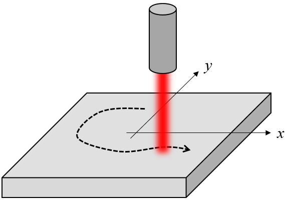
Schematic of a laser heat source traversing over a workpiece.
Now, let’s look at several different ways in which we can define the moving focus point to follow a known tool path.
Method 1: Using Variables
The simplest approach is to use a set of variables to define the position of the focus and distribution of the heat load over time. Let’s say that we want to have a 1-kW total heat load moving in a 40-cm radius circular path every 10 s. Furthermore, the heat load has a Gaussian intensity distribution with a 5-cm waist radius. We can define this information using variables, as shown in the screenshot below.
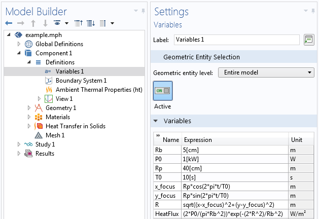
The first four definitions, Rb, P0, Rp, and T0, are actually just constants. If we would like to alter any of these definitions via a parametric sweep later on, we could also define them as Global Parameters. For now, it is simplest to just show them all in one place.
The next two variables, x_focus and y_focus, are not constant: They vary as a function of time, the built-in variable t. We can see that these variables describe a point moving on a circular path about the origin as:
Rp*cos(2*pi*t/T0)
Rp*sin(2*pi*t/T0)
The next variable, R, is a function of time and space. It makes use of the coordinate variables x and y, as well as x_focus and y_focus, which we just saw are functions of time. So at each instant in time and at every point in space, this variable tells us the distance (in the xy-plane) from the laser focal point.
The last variable, HeatFlux, is a function of R and the constants. It defines a Gaussian intensity profile about the focal point such that the total heat flux equals the defined power. It is this variable, HeatFlux, that we enter as a boundary condition, as shown in the screenshot below.
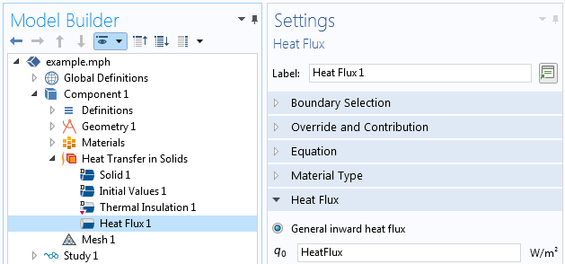
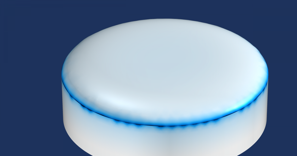
This prescribed heat flux expression then gives the heating profile path visualized below.
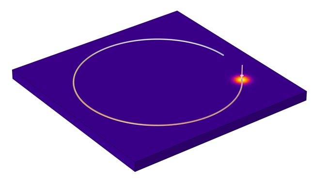
A circular heating profile set up via the Variables node.
Method 2: Using Interpolation Functions
So far, this isn’t very complicated; just a few expressions. But we can replace the simple expressions for x_focus and y_focus with something more general. COMSOL Multiphysics provides a variety of built-in functions in the software. For our discussion here, the most useful is the Interpolation function, which lets us read in data from a text file. Let’s suppose we have a text file containing rows of data of time and the x– and y-locations of the laser focus at that time. A sample of such a file is shown below:
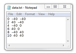
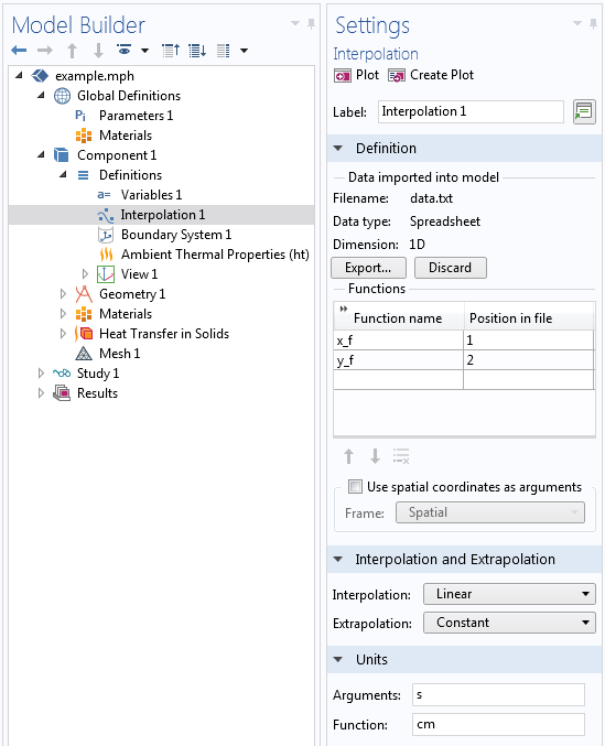
Such data can be read in to the Interpolation function using the settings shown below. Note that there is just a single argument here, time, and the two columns of data after that represent the x-focus and y-focus, respectively, in units of centimeters. Between the specified points in time, we want the laser to move linearly. We specify the function names as x_f and y_f, respectively, and make sure to set the arguments correctly.
We can then just alter our previous expressions for the focus to be x_focus = x_f(t) and y_focus = y_f(t) and get the moving load pictured below.
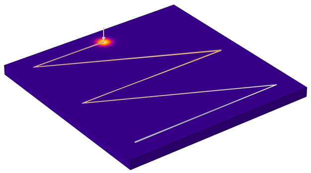
A heating profile read in from a text file.
We can see that this Interpolation function quickly lets us read in some very complicated profile patterns, we just need a way to generate these profiles and the text files. For example, the text file format used here is not too different from the G-code format, so if you have a heating path defined in such a format, it can be pretty simple to convert it to a COMSOL®-friendly input. On the other hand, maybe we would like to import a profile created in the ubiquitous 2D DXF file format. Let’s look at that next…
Method 3: Using Paths Imported from CAD Geometries
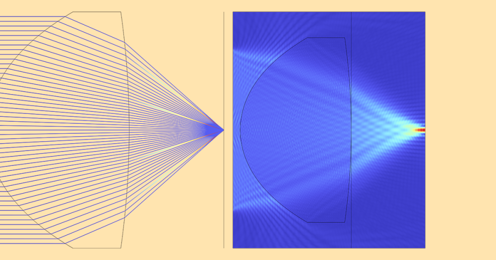
Suppose we want the load to move along a path we read in from an external file, as shown in the image below. We would like the laser to move smoothly along this path from one end to the other. Now, we need to do a bit more work.
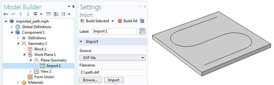
The S-shaped profile of the laser path is read in from a DXF file as a geometry.
The file that we’ve read in doesn’t have any information about time within it: It is just a path that we expect the laser to follow at a constant speed. Now, each edge of this imported path (and there may be thousands of edges) does have parameters s1 and s2 that vary linearly along the length, but if there are many edges, we probably wouldn’t want to work with these parameters. So instead, how do we compute where the laser is at every point in time along the entire set of lines? One way in which we can do this is by introducing another partial differential equation (PDE) to solve, along the desired set of lines. The PDE we want to solve is:
where \nabla_t refers to the tangential direction to the curve.
This PDE, along with the boundary conditions of u = 0 at one end of the path and u = 1 at the other end, will give us a field along the path that varies linearly from 0 to 1, which will be proportional to the total arc length of all of the edges. We can set this up using the Coefficient Form Edge PDE interface, as shown in the screenshots below. All coefficient terms other than the Diffusion Coefficient, c, are set to zero.


Left: Settings of the Coefficient Form Edge PDE interface needed to compute the path. Right: The diffusion coefficient term, c, is a constant; all other coefficients are set to zero.
Then, two Dirichlet boundary conditions set the field, u, at either ends, and we solve this PDE in a stationary step, prior to solving the heat transfer problem but still within the same study.
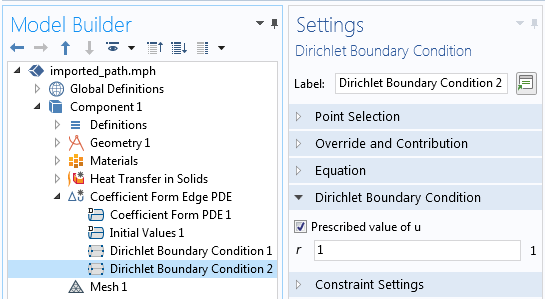
Two Dirichlet boundary conditions are used at the start and end of the profile path to constrain the field.
Next, we introduce a single minimum component coupling operator into the model, with the source selected as the edges to follow. This minimum operator is used to define the focal point coordinates, e.g.:
x_focus = minop1(abs(u-t/T0),x)
y_focus = minop1(abs(u-t/T0),y)
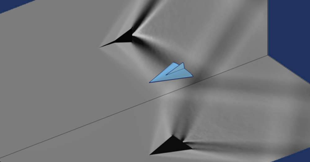
Note that the minimum operator is given two arguments. When we call the operator with two arguments, it will return the value of the second argument where the first argument is at a minimum. Thus, at each time, t, it will return the x– and y-locations of a point on the edge that is t/T0 fraction of the way from one end to the other.


Left: The minimum operator is defined over the path that the heat source follows. Right: The laser heat source following the path defined by an imported DXF file.
And what if we would like the laser to traverse different parts of the path at different speeds? We would just need to adjust the coefficient, c, along those sets of edges. Suppose we want the laser to move three times faster along the curved boundaries than along the straight lines: just make c three times larger. Note that the absolute value doesn’t matter, it is just the ratio of the coefficient magnitudes that matters. The one drawback to this approach arises when the path crosses itself. In that situation, you would need to subdivide the path into two, or more, groups of paths; solve a PDE on each; and do a bit more bookkeeping for the variables.
Closing Remarks on Modeling Moving Loads and Constraints
In this blog post, we have looked at three different approaches of modeling a moving load. To try them yourself, click the button below to head to the Application Gallery. There, you can download the MPH-files for the models featured above.
Several other examples within the Application Gallery also make use of these techniques, including:
Although in this blog post we only considered loads, note that we can also apply these techniques to constraints, as described in How to Make Boundary Conditions Conditional in Your Simulation.
Do you have further questions about using COMSOL Multiphysics for your modeling applications? Please let us know!


Comments (15)
Elif Demirbas
January 21, 2019Hi Walter,
I have a question related to laser power. In most of the laser heating tutorials, laser power is constant. Is it possible to define a varying laser power over time, for example like a gaussian function? And use this laser power function to heat the wafer. In the original laser heating wafer tutorial, the expression for the heat flux is p_laser[1/W]*gp1(x-wv1(t))*gp1(y) under the Analytic section. I tried replacing the p_laser with a gaussian function with an argument t, “gp2(t)*gp1(x-wv1(t))*gp1(y)”, however when I plot it, it plots over x and y only. How can I include the time dependency to the laser power?
Any information is much appreciated.
Thanks,
Elif
Walter Frei
January 22, 2019Hello Elif,
Yes, you can modify the power function to vary with time, just introduce a function that varies over time as well. See also: https://www.comsol.com/support/knowledgebase/1245/
Lyubo
July 20, 2020Can this laser be used to ablate the surface?
torikul islam piash
February 16, 2021did you made this laser which can ablate surface? I also want to construct this laser!
Long Wang
May 13, 2020Hi Walter,
What if I want to simulate the laser moving from an imported trajectory, and then a new layer is added above, and the laser is starting running on that new layer. This is a typical process of additive manufacturing. Since there is no birth and death mechanism of domains, how to enable another layer after one layer is fused?
Any hint?
Thanks,
Long
Sourav Mahato
January 12, 2023hey Long wang did you find the answer i need help regarding that too
MITHUN HARI
August 26, 2020Hi Walter,
I have a question related to acoustics. How can I add a sinusoidal load on a voice coil. ?
torikul islam piash
February 16, 2021I want to build a laser which can penetrate surface! can you suggest me how can I construct it?
Walter Frei
February 16, 2021 COMSOL EmployeeHello Torikul,
See also: https://www.comsol.com/blogs/modeling-laser-material-interactions-in-comsol-multiphysics/
Rakesh Sivakumar
September 2, 2021Is there any blog posts related to arc welding and additive manufacturing.
I am using double ellipsoidal heat source model. In that case how to include functions in the model
Alp Aydin
November 14, 2021Hi Walter,
SPEED of the beam on a particular path: could you clarify how to define it?
Raviraj Verma
August 25, 2022Hello Walter,
Could you please provide a little more about “Method 3: Using Paths Imported from CAD Geometries” to understand this approach in a much better way?
(I am using COMSOL Multiphysics 5.5)
Best!
Walter Frei
January 12, 2023 COMSOL EmployeeHello Raviraj,
You’ll find the example files, in version 6.0, associated with this article here:
https://www.comsol.com/model/modeling-of-moving-loads-69831
We do recommend that you upgrade to the current version of the software as well.
B Wheelz
January 17, 2024Hi Walter,
Thanks for these examples. These are tantalizing close to what I’m trying to do, but I can’t figure out the last step!
My heat function is defined by an interpolation function instead of parameterically. So I have one interpolation function F(x,y,z) describing the initial source (centered on zero), then two functions x(t) y(t) describing the focus. I have been scratching my head and I’m pretty sure there is no general way to combine these functions…right?
Perhaps the answer is that I make a parametric function F(x,y,z,t)? In other words let the interpolation handle everything?
Brendan
Walter Frei
January 17, 2024 COMSOL EmployeeHello Brendan,
This level of detail is a bit beyond the scope of what can be addressed in a comment, and is better to address via COMSOL Technical Support.
Best Regards,