

This is an introduction to the weak form for those of us who didn’t grow up using finite element analysis and vector calculus in our daily lives, but are nevertheless interested in learning about the weak form, with the help of some physical intuition and basic calculus.
About the Weak Form, Briefly
For many of the different types of physics simulated with COMSOL Multiphysics, a weak formulation, or weak form, is used behind the scenes to construct the mathematical model. Understanding the weak form will help us gain insight into how the COMSOL software works internally as well as enable us to write our own equations when there is no built-in interface available for the particular physics involved in our model.
You may also be interested in reading my colleague Bettina Schieche’s blog post “The Strength of the Weak Form“.
A Simple Example
Let’s consider a concrete example of 1D heat transfer at steady state with no heat source. Specifically, we are interested in the temperature, T, as a function of the position x in the domain defined by the interval $1\le x\le 5$. For simplicity, we assume the heat conductivity is unity. Then, the heat flux, q, in the positive x-direction is given by the gradient of the temperature T:
(1)
and the conservation of the heat flux (with no heat source in the domain) simply says
(2)
This is the main equation that we want to solve. Its solution will give us the temperature profile within the domain. Equations of this form appear in many different disciplines. For example, in electrostatics, T is replaced by the electric potential and q by the electric field, while in elasticity, T becomes the displacement and q becomes the stress.
Here, we start to see why COMSOL Multiphysics can solve coupled multiphysics problems in a breeze: No matter what physical mechanisms are involved, they are modeled by equations and once the equations are written down, they can be discretized and solved straightforwardly by the core algorithms of the COMSOL software.
Some readers may ask why we chose this seemingly too simple of an example, whose analytical solution can be easily obtained by very simple math or physical arguments. The reason is two-fold:
- We want to focus on the central idea of the weak form and not be distracted by the math of a complicated physical system.
- In subsequent posts, we will expand the example to more than one domain to demonstrate the coupling between two equation systems through their boundary conditions. Starting with a more complicated example now will almost certainly obscure the central theme later when the example is expanded.
The Weak Formulation
Equation (2) involves the first derivative of the heat flux, q, or the second derivative of the temperature, T, which may cause numerical issues in practical situations where the differentiability of the temperature profile may be limited. For example, at a boundary where the adjacent materials have different values of thermal conductivity, the first derivative of the temperature T becomes discontinuous and the second derivative of T can not be evaluated numerically. The main idea of the weak form is to turn the differential equation into an integral equation, so as to lessen the burden on the numerical algorithm in evaluating derivatives.
To turn the differential equation (2) into an integral equation, a naive first approach may be to integrate it over the entire domain $1\le x\le 5$:
This asks that the average value of $\partial_x q(x)$ in the entire domain is zero. Indeed, it seems “too weak” as compared to the original differential equation, which asks that $\partial_x q(x)$ should be zero everywhere in the interval $1\le x\le 5$. To improve upon it, we can ask instead that the average value of $\partial_x q(x)$ in a very narrow domain is zero, say,
The integral only involves the value of $\partial_x q(x)$ in the vicinity of x=3.5. Thus, the relation above requires it not to be too far away from zero: $\partial_x q(3.5) \approx 0$. Extending the same idea to all locations in the entire domain $1\le x\le 5$, we see that the original differential equation may be approximated by a set of integral equations, like this:
(3)
The higher the number of integral equations in the set, the better the approximation. In the limit of the infinite number of such integral equations, we recover the original differential equation. It is cumbersome or even impossible to write out all the integral equations in the set, but we can apply the same idea in a different way.
The main idea is to sample the value of $\partial_x q(x)$ in a narrow range. This is done by integrating it over a narrow range in Eq. (3) above. The same kind of sampling can be done by multiplying the integrand by a weight function \tilde{T}(x) that is non-trivial only in a narrow range, as shown pictorially below:
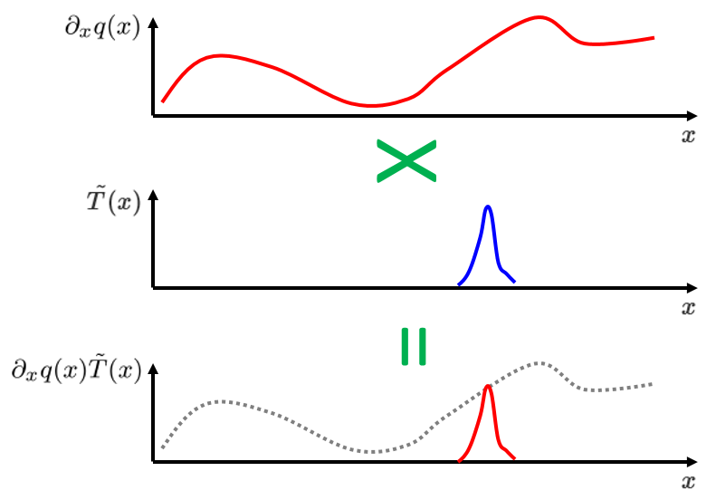
Then, we can integrate the product $\partial_x q(x)\tilde{T}(x)$ over the entire domain $1\le x\le 5$ for a variety of weight functions \tilde{T}(x). Each weight function limits the contribution of the integrand to a narrow range centered around a different x value, thus achieving the same effect as the collection of integral equations in Eq. (3). This leads us to the weak formulation, which states that the relation
(4)
should hold for a set of weight functions \tilde{T}(x), commonly called test functions. For every value of x, say x=3.5, we can choose a test function \tilde{T}(x) that is a narrow weight function centered around x=3.5. Plugging this test function into Eq. (4) would sample the value of $\partial_x q(x)$ in the vicinity of x=3.5 and so require it not to be too far away from zero: $\partial_x q(3.5) \approx 0$.
By plugging a large number of narrow weight functions as test functions into Eq. (4), each centered at a different location in the interval $1\le x\le 5$, the value of the function $\partial_x q(x)$ will be clamped down to zero everywhere within the domain.
Footnote: In the picture above, we intentionally plotted $\partial_x q(x)$ as an arbitrary curve, not the final solution to the equation, to emphasize the fact that we haven’t found the solution yet. Later on in the solution process, this arbitrary curve will be pushed up and down by a collection of test functions to reach the shape of the final solution.
Reducing Order of Differentiation
Note that the order of differentiation in the integrand of Eq. (4) is still the same as in Eq. (2) (after all, it’s the same function $\partial_x q(x)$), but it can be reduced using the method of integration by parts:
(5)
Now, there is no derivative of the heat flow, q, in the equation, or in terms of the temperature, T, the order of differentiation is reduced from two to one. What about the first derivative of the test function \tilde{T}(x), which just now appeared in the equation?
As we have seen in the previous section, the test function serves as a tool for us to find the solution to the equation. Thus, we have the freedom to choose any conveniently differentiable form for it.
Natural Boundary Condition
The first two terms of Eq. (5) involve the heat flux and test function at the domain boundaries x=1 and x=5, with the heat flux, q, defined in the positive x-direction. We can rewrite them in terms of the flux going out of the domain and move them to the right-hand side:
(6)
Here, $\Lambda$ is the outgoing flux, and the subscripts 1 and 2 represent the domain boundaries x=1 and x=5, respectively \Lambda_1\equiv -q(x=1) \mbox{, } \Lambda_2\equiv +q(x=5) \mbox{, } \tilde{T}_1\equiv \tilde{T}(x=1) \mbox{, } \tilde{T}_2\equiv \tilde{T}(x=5).
Also, we have used the heat flux relation (1) to write the integrand in terms of the temperature, T, and its test function, \tilde{T}. The right-hand side of the equation provides a natural way to assign boundary conditions in terms of the heat flux. The simplest is to set both \Lambda_1 and \Lambda_2 to zero to get insulating boundary conditions (no heat flux through the boundaries).
This is exactly the reason why in COMSOL Multiphysics the default boundary condition for heat transfer is “Thermal Insulation” and the one for solid mechanics is “Free (no boundary force)”. This kind of boundary condition, which specifies the flux or force (the first derivative of the variable being solved), is commonly called the natural boundary condition or the Neumann boundary condition.
Fixed Boundary Condition
Another type of boundary condition, commonly called the fixed boundary condition or the Dirichlet boundary condition, specifies the value of the variable being solved. In our current example, it specifies the value of the temperature at a point on the boundary. This kind of boundary condition is usually needed to set up a well-posed problem with a unique solution. For example, in fluid flow, we need to specify the pressure somewhere (not just the flow); and in solid mechanics, we need to specify the displacement somewhere (not just the force).
As we have seen in the example, the weak formulation provides a natural way to specify the heat flux at a boundary. How do we specify a fixed temperature at a boundary, then?
The trick is to take advantage of the mathematical structure of the natural boundary condition and apply the same idea of using test functions to clamp down the solution. Conceptually, to maintain a fixed temperature at a boundary point, a certain heat flux coming from the outside of the boundary is needed to compensate for the heat flux inside of the boundary. The weak formulation poses the problem as this: Find the heat flux needed to maintain the fixed temperature at the boundary point.
For example, if we want to specify the outgoing flux \Lambda to be 2 at x=1 and the temperature T to be 9 at x=5, then we introduce a new unknown variable \lambda_2 and its corresponding test function \tilde{\lambda}_2, and write Eq. (6) as:
(7)
Here, on the right-hand side, the first term specifies the outgoing flux of 2 at x=1 and the second term specifies the unknown flux at x=5; both terms come directly from the natural boundary condition terms on the right-hand side of Eq. (6).
The new variable \lambda_2 represents the unknown heat flux to be determined at the boundary x=5. The third term is added to the equation to force the solution to be T=9 at x=5 by means of the test function \tilde{\lambda}_2 in the same fashion as in the earlier discussion about the test function \tilde{T}(x).
Comment on Higher Dimensions
So far, we have been discussing a very simple one-dimensional example. In higher dimensions, such as a 2D surface domain or a 3D volume domain, the equations become more complicated, but the basic idea remains the same.
The weak formulation turns a differential equation into an integral equation. Integration by parts reduces the order of differentiation to provide numerical advantages, and generates natural boundary conditions for specifying fluxes at the boundaries. In the simple 1D example, the boundary is the two end points and the flux is a single value at each point.
In 2D and 3D, the boundary is the closed curve and the closed surface enclosing the domain, respectively. The right-hand side of Eq. (6) becomes the line or surface integral of the incoming flux density, in other words, the total incoming flux. In essence, the process of integration by parts in 2D and 3D uses the divergence theorem to obtain the line or surface integral of the flux at the boundary of the modeling domain.
In this blog post, we chose the simple 1D example so that the central idea wouldn’t be obscured by the complexity of the math.
Summary and Next Up
Today, we learned about the idea of the weak formulation of using test functions to clamp down the solution. Integrating the weak form by parts provides the numerical benefit of reduced differentiation order. It also provides a natural way to specify boundary conditions in terms of the fluxes or forces (the first derivatives of the variables being solved), the so-called natural boundary condition or the Neumann boundary condition.
When solving a practical problem, it’s often necessary to specify the variable being solved — not just its derivative — via the so-called fixed boundary condition or the Dirichlet boundary condition. We saw that the weak formulation uses the same mechanism of test functions and its natural boundary conditions to construct additional terms for the fixed boundary conditions.
So far, we have left the equations in their original analytical forms without any numerical approximation. In the next blog post, we will implement the weak form equation (7) in COMSOL Multiphysics to solve it numerically. After that, we will discuss how the numerical approximation is done internally, how the same problem can be solved in different ways, and how different boundary conditions can be set up for different types of problems.

Comments (31)
Felipe Beltran-Mejia
December 22, 2014Thank you Chien,
This is a great post!
I cant wait for your next post implementing all the theory exposed here.
—
Felipe.
Felipe Beltran-Mejia
December 22, 2014Just a small comment, I wouldn’t use T as a test function since your are already using it for temperature. Sometimes it is a bit confusing.
Thanks again,
—
Felipe.
Chien Liu
January 5, 2015Dear Felipe,
Thank you for your encouraging comments!
It is common to add a tilde (~) on top of the symbol to represent its test function, which is what we did here for the temperature function T. Could it be that somehow the tilde on top of the symbol “T” does not show up in your web browser? You should be able to see the tilde in the labels for the vertical axis in the drawing. The same tilde should be present in the text, for example, after “by a weight function” right before the drawing.
Happy new year!
Chien
Rogelio Hernandez Aguirre
January 27, 2015So far, the best explanation ever for the Weak form!!
Bravo!
Perry Gao
August 1, 2015Dear Chien,
Thanks for your great post!
I have a question about natural boundary conditions when implementing weak form in Comsol 4.3 .
In 4.3, the default boundary condition is zero flux, and is defined as:
‘dot(normal unit vector, flux)=0’. However I couldn’t find the definition of ‘flux’ here. Is it the gradiant of the dependent variables? or it is derived from the weak form I gave?
If it is the later one, how is it implemented?
Thanks again!
Chien Liu
August 3, 2015Dear Perry,
Thanks for the comments. The default zero flux boundary condition is implemented by “doing nothing” – in other words leaving the right hand side of Eq. (6) as zero. If there are more specific questions please do not hesitate to contact us at
support@comsol.com
Sincerely,
Chien
Perry Gao
November 10, 2015Dear Chien
Just wonna say thanks so much for your great articles and answers!
They are truely very helpful!
Best wishes,
Perry
Mohankumar Kambapalli
December 24, 2015Dear Chien,
Good article. I appreciate for keeping it simple and informative.
Well, I was wondering if there is a negative sign missing for the left term in equation 6 ?
Can u confirm, please?
Thanks.
Chien Liu
January 4, 2016Dear Mohankumar,
Happy new year! Thank you for the comment. There should not be a negative sign on the left hand side of Eq. (6) as you suggested. Remember that the heat flux and the temperature gradient are in opposite directions (see Eq. (1)). If there are still questions on this please contact us at
support@comsol.com
Sincerely,
Chien
wang shuo
March 13, 2016If a higher order shape function was applied, is it possible to write down the weak form without Reducing the order of differentiation? (Integration by parts)
Chien Liu
March 15, 2016Dear shuo,
If you find it more useful to not reducing the order of differentiation in your particular situation, then you are definitely not required to do so by any means.
Sincerely,
Chien
峰 程
April 6, 2016Dear Chien,

 .
.
Thanks for your article. I have some questions about it.
First, I can’t understand the derivation of Eq.(4). I think Eq.(4) should be written as
with
Here I used the Dirac delta function to replace the test function. It can be replaced by other “narrow” functions, but its strictness will be “weakened”.
Can you tell me a little more about the test function so I can relate it with the Dirac delta function?
Many thanks.
Sincerely,
Feng
Chien Liu
April 7, 2016Dear Feng,
It will become clear later in this blog:
https://www.comsol.com/blogs/discretizing-the-weak-form-equations/
why the Dirac delta function would not be a good choice as the test function for numerical analysis. Roughly speaking we need the basis function to have some finite width in order to reconstruct the solution function. For more in-depth discussion on this topic, you may want to take a look at the references listed in the comments of this blog:
https://www.comsol.com/blogs/implementing-the-weak-form-in-comsol-multiphysics/
Sincerely,
Chien
Jorge Yannie
April 17, 2016Hello Chien,
I want to thank you for such a great post! Clear and to the point without missing the central idea with complex mathematical language and equations. Great job and keep it flowing!
Loving Comsol!
Regards,
Jorge
Khoa Phan
September 29, 2016My browser Chrome just won’t display mathematical formula correctly. Can anyone tell me how to fix this?
Khoa Phan
September 29, 2016My browser just won’t display the mathematical formula correctly. COuld some please tell me how to fix?
Chien Liu
September 29, 2016Dear Khoa, Thanks for the comments. If you meant the LaTeX in the comment posted by Feng, our web team has fixed it now. If you meant something else, could you please specify exactly what the problem is? Thanks! Chien
Khoa Phan
September 30, 2016Thank you very much for your respond. I can see correctly now
Alwar Samy Ramasamy
July 17, 2018Dear Chien,
Thanks for giving a easy intro to weak form.
I have a doubt in equation 7, how do you get the third term in RHS which states T=9 at x=5. How that is attained?
Can you please clarify
Chien Liu
July 18, 2018Dear Alwar, Thank you for the question. One way to think about this is to consider a problem of constrained optimization. Then the last two terms in equation 7 come from taking the variation operation on the product of the Lagrange multiplier (labmda_2) and the constraint (T_2-9). Sincerely, Chien
George Beeler
October 1, 2018Better explanation than the textbooks I have read on the subject. I do feel it is a bit unfortunate to call this a weak formulation as it is a very powerful way to solve PDEs without the inherent fluctuations of the direct discretization.
I presume this is the form that COMSOL uses in the Implicit formulation Solver vs. Direct Solver, or am I missing another axis in the solution methodology?
Chien Liu
October 2, 2018Dear George,
Thank you for the comments. For solver related topics, you can check out the blog series on solvers:
http://www.comsol.com/blogs/tag/solver-series/
Sincerely,
Chien
Lucas Cui
November 9, 2019Hello Chien,
Nice article! In COMSOL the default flux at boundaries is zero, but sometimes the flux is not zero so we have to insert a weak contribution to input the actual value, as you explained in the blog. My question is: if I input the new value of the flux by weak contribution, will the default zero flux condition be suppressed?
Many thanks.
Lucas
Chien Liu
November 9, 2019 COMSOL EmployeeDear Lucas, Thank you for the comments. The weak contribution is accumulative — two contributions on the same boundary are summed up, not replacing/suppressing each other. Of course for the default zero flux condition the effect is the same (either adding or replacing). However for non-zero contributions, they are added together, not replacing each other. Sincerely, Chien
Shahrzad Molavi
May 22, 2020Thank you so much for your useful blogs. It helped me a lot.
Xuan mu
October 18, 2020Really helpful blog! Thank you, Dr. Chein Liu.
Jishnu Goswami
July 5, 2022Very very good post for anyone starting simulating in COMSOL. Thanks for the informative post
yeongik jang
July 12, 2023Dear Chien,
Thanks for your post!
Can you elaborate a bit more on the process of going from equation (6) to equation (7)?
I understand the application of boundary conditions at x = 1,
I don’t understand how to apply the Lagrange multiplier to make the last two terms.(boundary condition at x=5)
I would appreciate it if you could elaborate a bit more on the process of applying the Lagrangian multiplier to get to the last two terms.
thank you!
Jung-Hwan Lee
February 16, 2024Thank you for your great explanation.
From (6) on the right side, =- A1T1 – A2T2 is correct? or should be changed = -A1T1 + A2T2
Small minor question. Thank you ^^
Taofik Nassan
April 23, 2024No. Your correction is not valid. Equation (6) is completely correct due to constant selection sign:)
Taofik
Computational Modeling Expert
February 23, 2024Dear Chien, thanks for this awesome explanation! 😀 It helped me so much when I was a student studying PDEs. Your post even inspired me to make a YouTube video about the weak formulation ten years later. Check it out if you are interested:
https://youtu.be/xZpESocdvn4