
To help understand the complicated universe we live in, we have traditionally compartmentalized physics phenomena into distinct disciplinary specializations. However, natural and engineering problems often cross these utilitarian borders. A major strength of the COMSOL Multiphysics® software is how easily such cross-disciplinary interactions, which we refer to as multiphysics interactions, can be accounted for. The COMSOL® software provides a plethora of built-in multiphysics couplings and even enables you to implement your own physics couplings. Learn about our three-part Learning Center course on this topic below…
Multiple Physics, Multiple Approaches
When adding the physics for a multiphysics model, there are a number of ways in which you can handle the physics setup. In COMSOL Multiphysics, there are three different approaches:
- Fully automatic
- Manual with predefined couplings
- Manual with user-defined couplings
In our new Learning Center course, Defining Multiphysics Models, one approach is covered in each respective part of the course, in the order outlined above. Each approach is advantageous for different modeling scenarios and varies in terms of ease of implementation and amount of effort required from the user.
We begin the course by discussing and showing the automated implementation, which is the most convenient and ideal to use in any case. It is especially helpful if you are just getting started with adding the physics for a multiphysics model. From there, we progressively move into more and more manual implementations, which typically require more time; work; and in some instances, intimate knowledge of the equation formulation of the physics involved.
During the course, we demonstrate the use of all three approaches using the same example: a thermal-electrical-mechanical (“tem”) version of the thermal microactuator tutorial model found in the Application Gallery on the COMSOL website. This demonstration accomplishes two things:
- Enables you to become knowledgeable in and comfortable working with the example model used
- Allows you to gain insight into the various ways that the physics can be coupled, after experiencing a small sample of these various ways
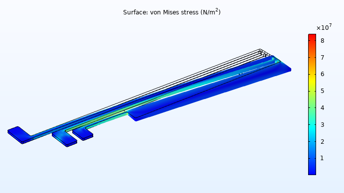
A plot of the stress results for the thermal microactuator tutorial model, which is the example used throughout the course.
Automate Your Multiphysics Model Setup
In the first part of the course, we introduce the fully automatic approach. The use of this approach requires the least amount of steps and effort on your behalf.
By automatic, we mean to use the predefined multiphysics interfaces readily available in COMSOL Multiphysics, as well as automatically preconfigured settings for the multiphysics interactions being simulated. This includes the solvers used when computing the model and the default plots generated for the solution. Adding these interfaces to your model makes the modeling process simple, since their use automatically adds the necessary physics interfaces and multiphysics coupling features to your model all at once.
In Part 1 of the Learning Center course, we discuss how the automatic approach lets you more quickly dive into defining the physics for a multiphysics model without being hampered by all the details. We also introduce the aforementioned example that is used throughout the course; the thermal microactuator tutorial model.
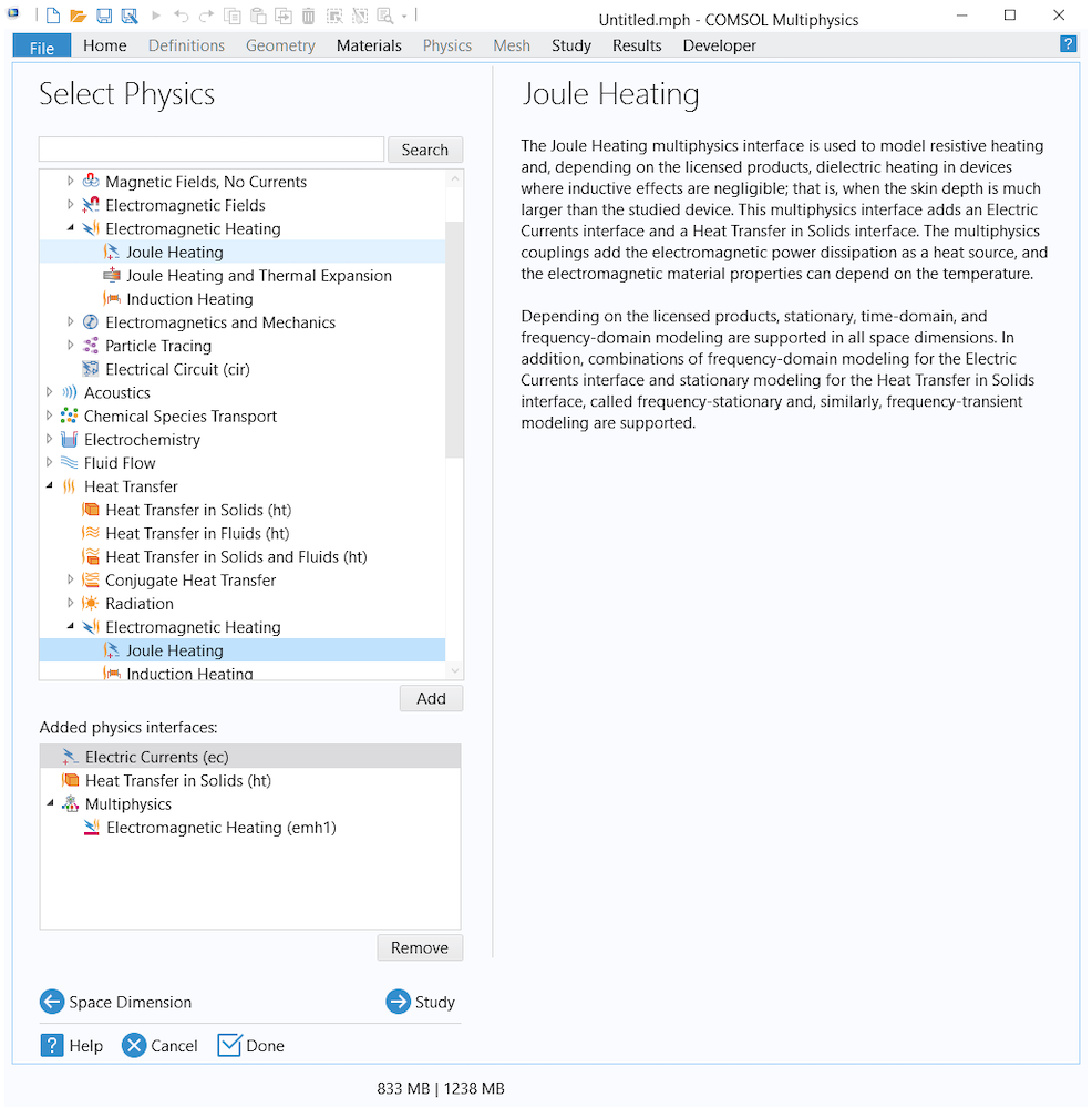
The Select Physics window, wherein a multiphysics interface has been added to the model. Done through use of the Model Wizard.
Define One Physics Phenomena at a Time
In Part 2 of the course, we introduce the manual approach with predefined couplings.
When modeling multiple physical phenomena, your simulation can be computationally expensive, depending on the spatial dimension, size of mesh elements, and number of physics interfaces involved, among other factors. Computing such a model can become even more time consuming if you encounter solver errors or want to change any of the physics settings and then recompute the model.
These potential setbacks can be minimized if not entirely eliminated through using an incremental methodology that is logically ordered according to the physics involved and the multiphysics interaction being simulated. This is why this modeling strategy is referred to as the manual approach with predefined couplings. Your multiphysics simulation is broken up into multiple studies as you incrementally add and build upon each physics interface one-by-one gradually, until you have reached the scope of the full multiphysics problem.
This approach is advantageous for many reasons. It enables you to narrow your focus on one physics interface or combination of physics interfaces at a time. However, it does require more steps and effort to implement before you reach the full multiphysics model setup and solution.
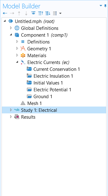
The model tree for the resistive heating of the thermal microactuator, using the manual with predefined couplings approach.
Utilize Flexibility for the Physics You Need
In Part 3, we explore how you should approach defining the physics for your multiphysics model when there are no predefined multiphysics interfaces or multiphysics couplings available for your combination of physics interfaces. In cases like these, you can manually administer coupling between the different physics interfaces in your model. We refer to this as the manual approach with user-defined couplings, since you add the respective physics interfaces and manually implement custom, user-defined multiphysics couplings.
In this approach, the flexibility of COMSOL Multiphysics truly shines, as there are many various ways you can manually couple the physics interfaces in your model, including:
- Domain source features, loads, and constraints
- Conservation law nodes
- Material properties
- Model inputs
- Boundary conditions and constraints
- Initial conditions
- Equation View nodes
- Derived variables
- User-defined expressions
It should be noted, however, that out of all of the approaches discussed thus far, this one requires the most effort to implement as well as an understanding of the equations and how the equation contribution for the multiphysics interaction should be defined.
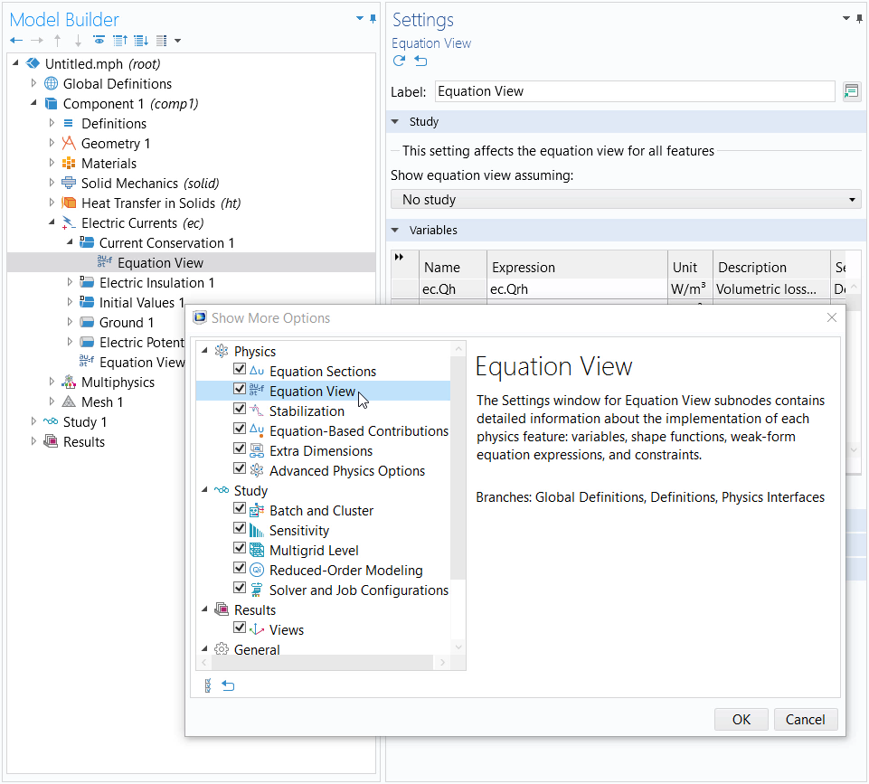
The model tree with the Equation View node displayed, which was enabled through the Show More Options dialog box.
Speed Up the Model Building Process
Upon completion of the Learning Center course, you will learn how to speed up your model building by:
- Taking advantage of the multiphysics interfaces and coupling options available in the COMSOL® software
- Expediting the troubleshooting of your multiphysics model through employing an incremental model build
- Following the guidance established in the course for handling custom, user-defined expressions for coupling between different physics interfaces
Read and watch the contents contained in the course to gain a comprehensive introduction to the automatic approach, manual approach with predefined couplings, and manual approach with user-defined couplings:
Stay tuned for future parts of this course to be added that will continue to expand upon the various capabilities and ways that you can couple multiple physical phenomena for a simulation in COMSOL Multiphysics. Happy modeling!


Comments (0)