

Global modeling of plasmas is a powerful approach to study large chemistry sets. In these models, the reactions are represented by rate coefficients. In particular, the rate coefficients of electron impact collisions depend on the electron energy distribution function (EEDF), which is often non-Mawellian and can be computed from an approximation of the Boltzmann equation (BE). Here, we explain how to create a global model fully coupled with the BE in the two-term approximation using the COMSOL Multiphysics® software.
Setting Up a Global Model of a Non-Maxwellian Discharge
The equations in a global model are greatly simplified because the spatial information of the different quantities in the plasma reactor is treated as volume-averaged. Without the spatial derivatives, the numerical solution of the equation set becomes considerably simpler and the computational time is reduced. Consequently, this type of model is useful when investigating a broad region of parameters for plasmas with complex chemistries.
For a closed reactor without net mass creation at the surfaces, a mixture of k=1,\dotsc,Q species and j=1,\dotsc,N reactions is described by the mass fraction balance equations for Q-1 species
where V is the reactor volume, \rho is the mass density, w_k is the mass fraction of species k, A_l is the area of surface l, h_l is a correction factor of surface l, R_s is the surface rate expression of surface l, R_k is the volume rate expression for species k, and M_k is the molar mass.
The sum in the last term is over surfaces where species are lost or created. One of the species mass fractions is found from mass conservation.
The electron number density is obtained from the electron neutrality condition
where n_k is the number density and Z_k is the charge number. The electron energy density, n_{\varepsilon}, can be computed from
+\sum_l \sum_{ions} e h_l \frac{A_l}{V}R_{surf,k,l} N_A \left( \varepsilon_e + \varepsilon_i \right)
where n_{\varepsilon}=n_e \overline \varepsilon, \overline \varepsilon is the mean electron energy, P_{abs} is the power absorbed by the plasma, and e is the elementary charge. The last term on the right-hand side accounts for the kinetic energy transported to the surface by electrons and ions. The summation is over all positive ions and boundaries with surface reactions, \varepsilon_e is the mean kinetic energy lost per electron lost, \varepsilon_i is the mean kinetic energy lost per ion lost, and N_A is Avogadro’s number.
In the equations above, the source terms R_k and R_{\varepsilon} are computed using rate coefficients that represent the effect of collisions. In particular, for electron impact collisions, the rate coefficients depend on the EEDF, which is often a non-Maxwellian distribution and depends on the discharge conditions. In practice, the EEDF can be obtained by solving an approximation of the electron BE using fundamental collision cross-section data. Once the EEDF is known, the rate coefficients are computed by a suitable averaging of the electron impact cross sections over the EEDF.
Describing the Boltzmann Equation and Two-Term Approximation
The BE that describes the evolution of an ensemble of electrons in a six-dimensional phase space is
where f is the EEDF, \textbf{v} is the velocity coordinates, m is the electron mass, \textbf{E} is the electric field, \nabla_v is the velocity gradient operators, and C is the rate of change in f due to collisions.
Normally, a rather simplified BE is solved instead. It is assumed that the electric field and the collision probabilities are spatially uniform. The BE is then written in terms of spherical coordinates in the velocity space and f is expanded in spherical harmonics. The series is truncated after the second term, and the so-called two-term approximation of f is
where f_0 is the isotropic part of f, f_1 is an anisotropic perturbation, v is the magnitude of the velocity, \theta is the angle between the velocity and the field direction, and z is the position along this direction.
The problem is further simplified by solving only steady-state cases where the electric field and EEDF are either stationary or oscillate at a high frequency. The last piece of simplification consists of separating the energy dependence of the EEDF from its time and space dependence using
where F_{0,1} is an energy distribution function constant in time and space that verifies the following normalization
where \gamma=\sqrt{2e/m} and \varepsilon = \left( v / \gamma \right)^2.
Using the above-mentioned approximations and after some manipulations, the equation for F_0 can be written in the form of a 1D convection-diffusion-reaction equation
(For more details, see Ref. 1.)
This equation can be used to compute an EEDF, providing a set of electron collision cross sections and a reduced electric field, E/N (ratio of the electric field strength to the gas number density). Depending on the operating conditions, it might be necessary to include the effect of superelastic collisions and electron-electron collisions. Quite often, the input quantity of interest is the mean electron energy. In this case, a Lagrange multiplier is introduced to solve for the reduced electric field such that the equation below is satisfied.
Once the EEDF is computed, the rate coefficients needed for a plasma global model are computed from
where \sigma_k is the cross section of reaction k.
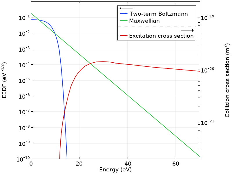
The figure below plots a computed EEDF obtained for argon at \overline{\varepsilon} = 5 eV and a corresponding Maxwellian. Note how the computed EEDF strongly deviates from a Maxwellian and how sharply it falls above the first excitation level of argon at 11.5 eV. In the same figure, the cross section for the excitation of the lumped level (corresponding to the first 4-s levels of argon) is plotted. With the information in this figure, the rate coefficient for the excitation of the 4-s levels can be computed.
Also important to note from this figure is that the computed EEDF and the cross section vary by several orders of magnitude in the overlapping region. In consequence, a small variation in \overline{\varepsilon} (or E/N) causes a large change in the rate coefficients. This example is for argon, but the same behavior is found in many other gases, and it is one of the reasons why plasmas have very nonlinear behavior.
In a practical application, the BE in the two-term approximation can be solved to provide rate coefficients to a global model. In such cases, the EEDF is computed every time the input conditions for the BE have changed.
Coupling the Global Model with the BE in the Two-Term Approximation
In this section, we show how to make a global model fully coupled with the BE in the two-term approximation using COMSOL Multiphysics. A three-step procedure is advised:
- Create a global model where an analytic EEDF is used
- Use the EEDF Initialization study to solve only for the EEDF
- Solve the fully coupled problem
Creating an EEDF Initialization Study
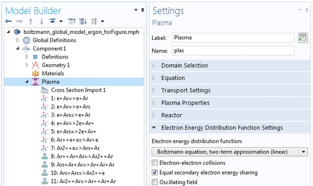
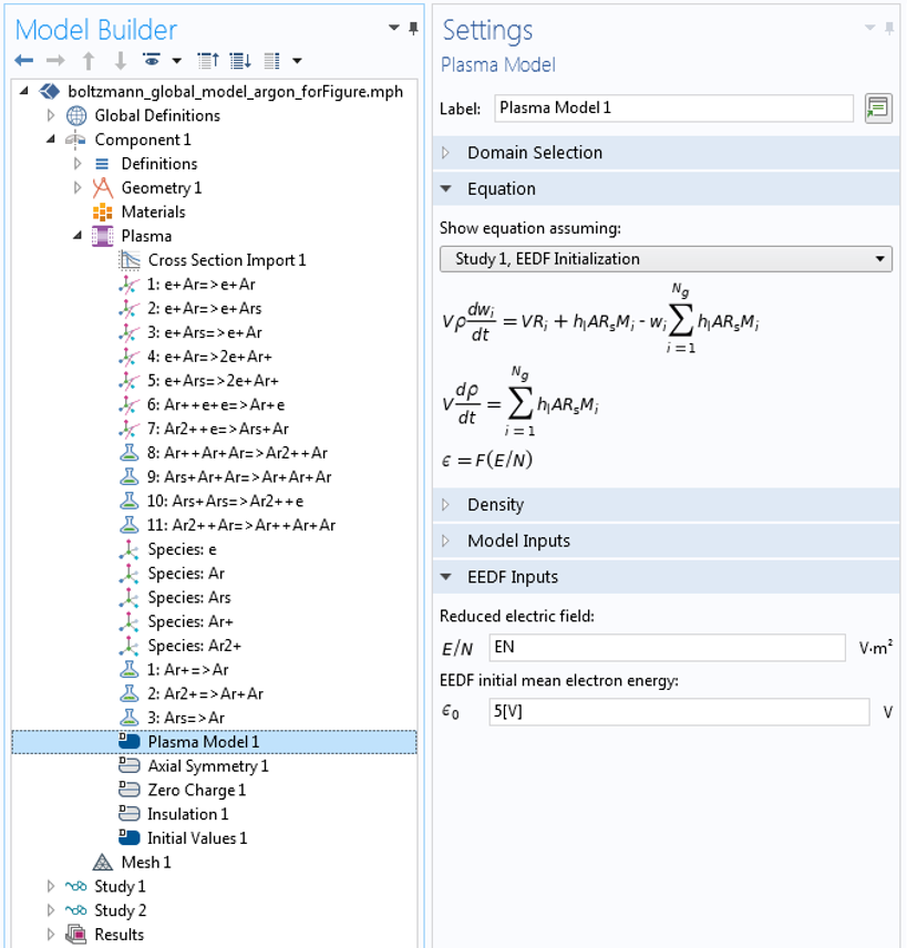
After having the global model working for an analytic EEDF (step 1), you can decide to investigate further to see if the EEDF used is suitable for your needs. You can do this by using an EEDF Initialization study to solve the BE in the two-term approximation. This study solves the BE for the electron impact cross sections provided and a choice of the reduced electric field or the mean electron energy. This procedure is exemplified in the screenshots below. First, select the Boltzmann equation, two-term approximation (linear) option — or the Boltzmann equation, two-term approximation (quadratic) option — in the Electron Energy Distribution Function Settings section.
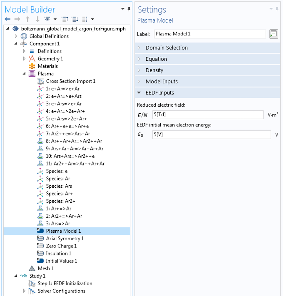
Then, set the Reduced electric field so that it’s used in the solution of the EEDF.
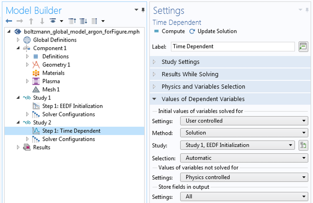
At this stage, you can compare the computed EEDF and the rate coefficients with the ones you used in the global model in step 1 and assess if the model needs further improvements. If you decide to solve the fully coupled problem, add another study and use the solution of the EEDF Initialization study as the initial condition, as shown below. Using the solution from the EEDF Initialization study is a requirement.
Coupling the Global Model Equations and BE
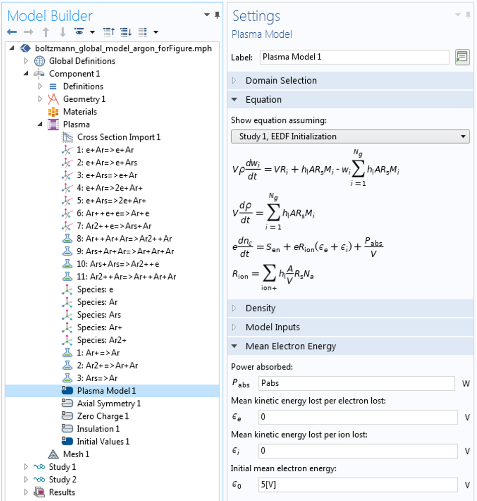
The coupling between the global model equations and the BE can happen in two different ways, depending on whether you use the Local field approximation or the Local energy approximation to define the mean electron energy in the Plasma Properties section. When using the Local field approximation, the excitation of the system is given from a reduced field. This electric field can be constant (a parameterization can be made over E/N) or can come from a solution of an equation (e.g., a circuit equation). When using the Local energy approximation, the global model equation for the electron mean energy is solved and the power absorbed by the plasma needs to be set by the user. In this case, the E/N is found so that the equation below is satisfied.
Example: A Plasma Sustained by a Direct Current Voltage Source
As a practical example, we chose to model an argon plasma created within a 4-mm gap by a direct current (DC) voltage source of 1 kV in series with a 100-kΩ resistance at 100 mTorr. This model is inspired by Ref. 2. We emphasize that the model has no spatial description and that geometrical parameters and volume-averaged quantities are used to describe the plasma in the gap. The voltage applied to the plasma, V_p, comes from the circuit equation
where V_{dc} is the applied voltage and R is the circuit resistance.
The plasma current, I_p, is computed from
where A is the plasma cross-sectional area and \mu N is the reduced electron mobility.
Solving for E/N, we obtain
where d is the gap distance between electrodes.
If we choose to use the Local field approximation, the equation for E/N above can be used directly in the EEDF Inputs section, as shown in the screenshot below.
If we choose to use the Local energy approximation, the power absorbed by the plasma can be defined as
in the Mean Electron Energy section, as in the screenshot below.
In this model, both approaches give very similar results, since the same electron energy loss/gain from collision events is accounted for in the BE and the mean electron energy equation, and because no energy losses to the wall are included in the mean electron energy equation.
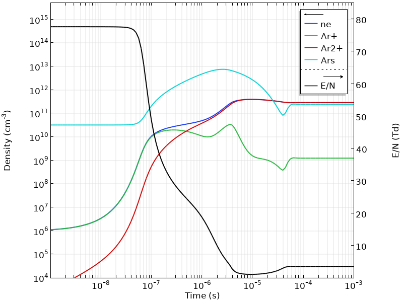
In the figure below, the temporal evolution of the charged species and the reduced electric field are shown. Initially, there is no plasma in the gap and the electric field (black line, right axis) maintains a constant value. When breakdown starts to occur, there is a rapid increase of the charged carriers and the current flowing into the circuit, resulting in a voltage drop across the gap. After this transient regime, a steady state is reached where the plasma is sustained with a reduced electric field of only 4 Td.
The temporal evolution of the EEDF is presented below. Initially, the EEDF has a large population above 15 eV, as it is necessary to facilitate the plasma breakdown. After the plasma formation, and due to the decrease of the electric field, the electron population cools down and the EEDF develops a tail with a steeper slope. As time progresses, and with the increase of the argon excited-state density, the influence of the superelastic reactions in the EEDF becomes noticeable, with the appearance of a bump at the high-energy end. Note that the time variation is presented on a log scale in this animation.
Next Steps
To try the example featured in this blog post, click the button below. Doing so will take you to the Application Gallery, where you can download the MPH-file for the model in addition to the step-by-step documentation.
You can also read more about modeling plasma physics in the following blog posts:
- Introduction to Plasma Modeling with Non-Maxwellian EEDFs
- The Boltzmann Equation, Two-Term Approximation Interface
- Electron Energy Distribution Function
References
- G.J.M. Hagelaar and L.C. Pitchford, “Solving the Boltzmann equation to obtain electron transport coefficients and rate coefficients for fluid models,” Plasma Sources Science and Technology, vol. 14, pp. 722–733, 2005.
- S. Pancheshnyi, B. Eismann, G. Hagelaar, and L. Pitchford, “ZDPlasKin: A New Tool for Plasmachemical Simulations”, The Eleventh International Symposium on High Pressure, Low Temperature Plasma Chemistry, 2008.

Comments (2)
Engr Hameed ullah
April 22, 2020Hello Sir
I am Engr Hameed Ullah from North China Electric Power University Beijing. can I ask something for you, sir. Kindly reply to me I will very thank full to you for this. Sir, I am reading your Ph.D. Student thesis ( Charge Transport and Breakdown Physics in
Liquid/Solid Insulation Systems by Joya Jadidian).
Sir can you guide me about these Simulations of Electrical streamers because I want to work on it further sir. Kindly help me, please, please
khalid hussain
September 10, 2021Hello Sir
I am Engr Hameed Ullah from North China Electric Power University Beijing. can I ask something for you, sir. Kindly reply to me I will very thank full to you for this. Sir, I am reading your Ph.D. Student thesis ( Charge Transport and Breakdown Physics in
Liquid/Solid Insulation Systems by Joya Jadidian).
Sir can you guide me about these Simulations of Electrical streamers because I want to work on it further sir. Kindly help me, please, please