

In 1875, John Kerr placed current-carrying coils in holes on either side of a glass slab, which created an electric field. After a polarized beam of light passed through the slab, he noticed that the polarization was different. This difference is related to the change in the glass’ refractive index, which is proportional to the square of the electric field — a phenomenon called the Kerr effect. See how to model this effect and other linear and nonlinear phenomena.
Understanding the Susceptibility of Nonlinear Optical Materials
When an electromagnetic field is applied to a dielectric material, the field displaces the material’s electron from its original orbit, making the electron oscillate at a particular frequency. In other words, the field polarizes the material. The displacement field in this case is represented as a function of the applied electric field as follows:
where E is the applied electric field vector, P is the induced polarization vector, \epsilon_0 is the vacuum permittivity, and \chi_0 is the isotropic susceptibility.
In the case of an anisotropic dielectric material, the induced polarization vector is a function of the susceptibility tensor as follows:
\chi_{11} & \chi_{12} & \chi_{13} \\
\chi_{21} & \chi_{22} & \chi_{23} \\
\chi_{31} & \chi_{32} & \chi_{33}
\end{bmatrix} \textbf{E}
Finally, in the case of a nonlinear dielectric material, the induced polarization can be expressed as a function of the electric field within the medium through the susceptibility (\chi) of the medium and, using a power series expansion, as follows:
where E is the applied electric field, ε0 is the vacuum permittivity, and \chi^{(i)} is the ith-order susceptibility.
It is assumed that there is no polarization that is independent of E. To have a thorough derivation of the polarization with nonlinear terms, refer to the book by Y. R. Shen (Ref. 5).
First-Order Susceptibility of Optical Materials
First-order susceptibility (\chi^{(1)}) deals with the change in refractive index due to the dipole oscillation of the bound and free carriers, such as electrons. Hendrik Lorentz originally came up with the idea of creating a mathematical oscillator model that can relate the dipole oscillation of bound electrons to the susceptibility of the material. Paul Drude originated the idea of oscillation within semiconductors, which deals with free carriers within the material. After combining the effects of bound and free carriers, the new model was called the Drude-Lorentz model.
In the COMSOL Multiphysics® software, the Drude-Lorentz model can be used to define the relative permittivity of a material. To define the Drude-Lorentz model, the relative permittivity at high frequency, plasma frequency, resonance frequency, and damping coefficient need to be given as inputs, as shown below. Multiple oscillators can also be added while assigning each of the oscillators’ contributions.
where εr is the complex relative permittivity of the material, ε∞ is the interband transition contribution to the permittivity, ωp is the plasma frequency, and Γ is the damping coefficient.
Modeling a Plasmonic Waveguide Filter
To showcase the capability of COMSOL Multiphysics in modeling the Drude-Lorentz material model, a waveguide with a metal-insulator-metal (MIM) interface is modeled. Here, the metal and insulator are modeled as silver and air, respectively. In this configuration, the width of the insulator is made to periodically vary along the waveguide (see the figure below). This particular arrangement of the insulator causes the waveguide to work like a filter known as a plasmonic waveguide filter.
This example shows that the waveguide rejects the electromagnetic radiation of the wavelength between 1.4 um and 1.6 um, but allows the rest of the wavelength (see the figure below). The silver material can be modeled using the Drude-Lorentz approximation, with ε∞ = 3.7, ωp = 13.8 rad/s, and Γ = 2.736 rad/s, while the insulator is modeled using air. As an alternative to the Drude-Lorentz material model approximation, the material property determined by Johnson and Christy’s experimental data (Ref. 4), which is available in the Material Library as Ag (Johnson), can be used.
Note that the output characteristic of this plasmonic waveguide filter is similar to that of the fiber Bragg grating (FBG) configuration.
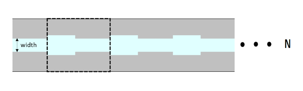
Schematic of the plasmonic waveguide filter. Blue and gray are the insulator and metal domain, respectively. The dashed line depicts a unit cell that is periodically repeated.
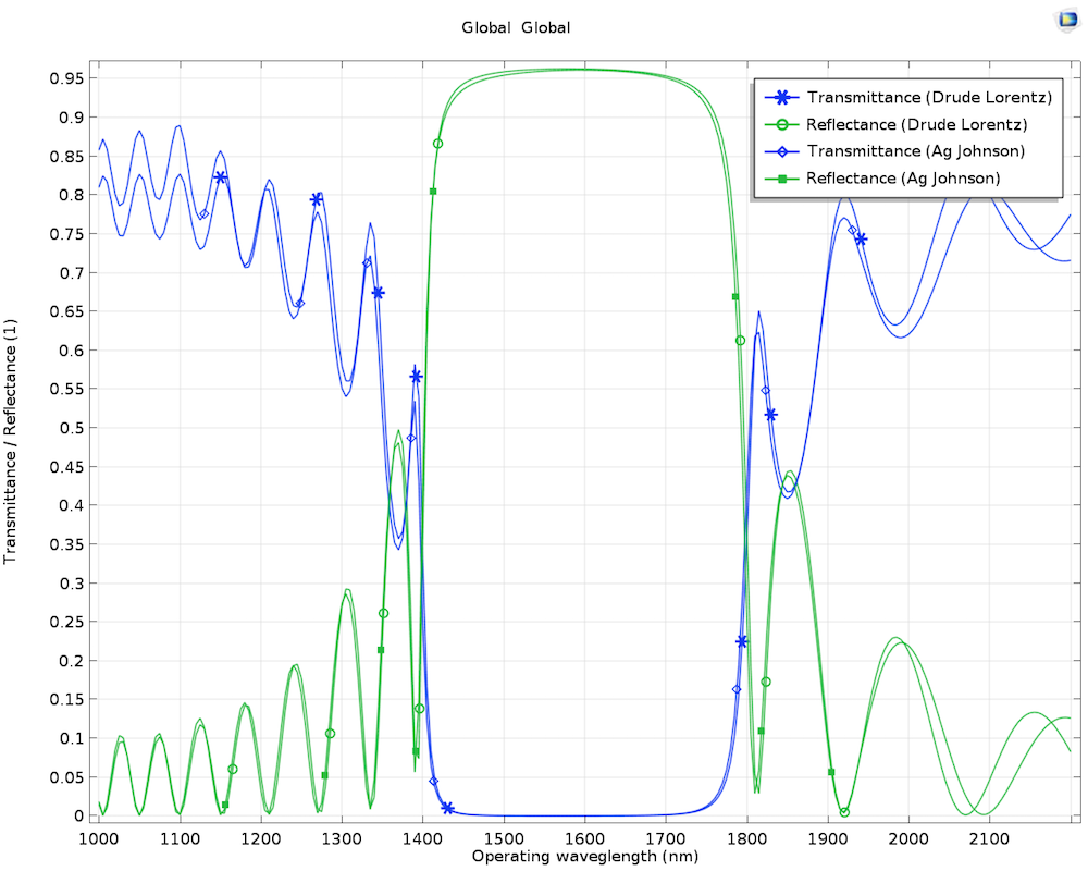
The transmittance and reflectance through the plasmonic grating filter (with 10 unit cells) using both the Drude-Lorentz model and Ag (Johnson) from the Material Library. You can download the MPH-file for this model from the Application Gallery.
Second-Order Susceptibility of Optical Materials
There are nonlinear crystals that display relatively high second-order susceptibility (\chi^{(2)}). When a monochromatic beam of light is introduced and passes through such a nonlinear crystal, not only does the output frequency spectrum show the original frequency (ω), but it also indicates the second-order harmonic frequency (2ω). Hence, this phenomenon is called second-harmonic generation (SHG).
The application of SHG lies in the field of laser design and engineering, where it’s challenging to find a material to eject light with shorter wavelengths. For example, when an infrared light source (1064 nm) is pumped through a potassium-dihydrogen-phosphate (KDP) crystal, the crystal ejects a green (532 nm) source of laser light.
In COMSOL Multiphysics, this approach can be modeled either with a transient or frequency-domain analysis in which the polarization is defined using the nonlinear coefficient (d), as shown below. In the transient analysis of the beam, the electric-field-dependent nonlinearity term needs to be introduced to the electric displacement field (D). The way it is introduced in this model is by clever use of the remnant electric displacement (Dr). As a matter of fact, the remnant electric displacement can also accept a nonlinear field quantity, which involves the square of one of the electric field components here. This approach displays the sum frequency generation as well as the difference frequency generation.
where D_r = d_{33} E_{z}^2, d_{33} is the nonlinear coefficient, and Ez is the z-component of the electric field.
With the frequency-domain analysis of the beam, only one particular frequency can be analyzed at one instance. (In other words, only one frequency can be analyzed with the Helmholtz equation.) Hence, the model sets up two interfaces and couples the two physics. The first interface represents the fundamental wave, while the second interface represents the second-harmonic frequency. The polarization of the first interface, P_{1y}, and that of the second interface, P_{2y}, can be defined as the following:
where d is the nonlinear coefficient, E_{1y} is the y-component of the electric field at the fundamental frequency, and E_{2y} is the y-component of the electric field at the second-harmonic frequency.
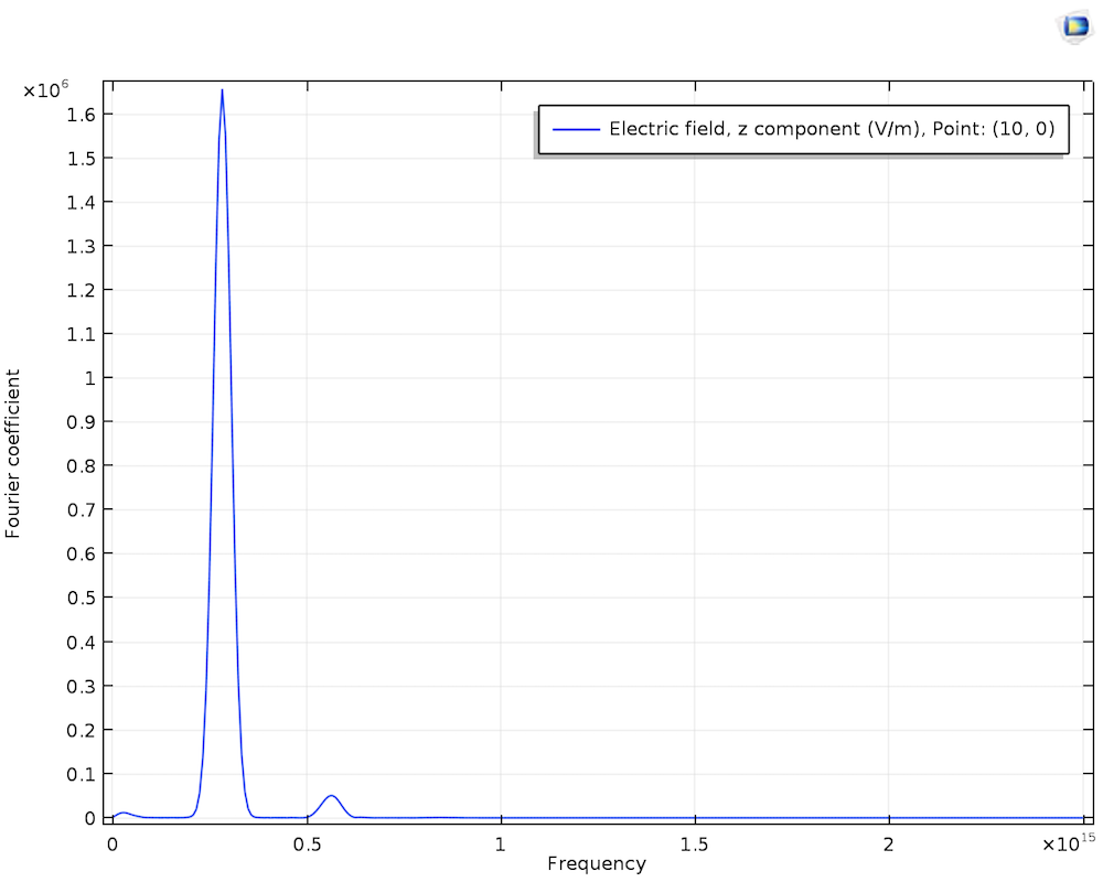
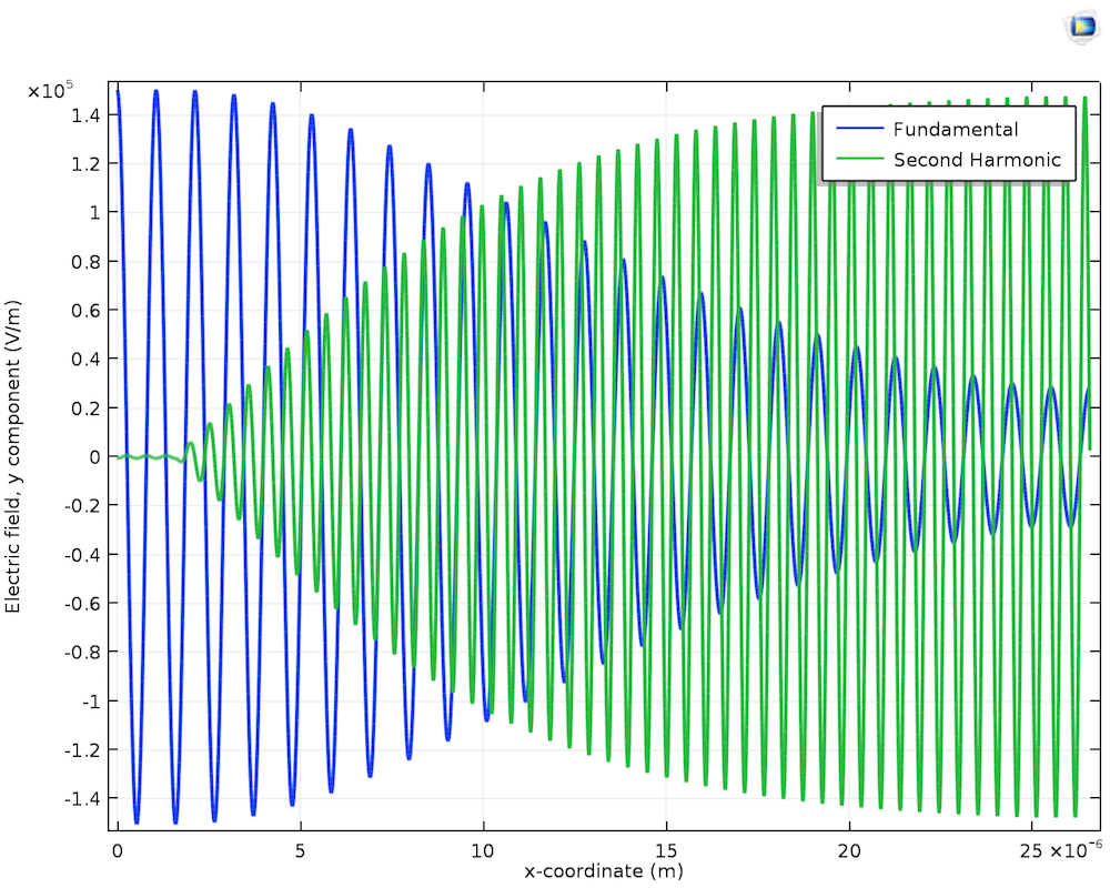
Left: The output frequency spectrum. The small peak on the left side of the large peak shows the difference frequency generation, while the small peak on the right shows the SHG. Right: The y-components of the electric fields for the fundamental and second-harmonic wave.
Third-Order Susceptibility of Optical Materials
The materials that have dominant third-order susceptibility (\chi^{(3)}) display phenomena such as the optical Kerr effect, self-phase modulation, cross-phase modulation, third-harmonic generation, and four-wave mixing. To illustrate the optical Kerr effect in COMSOL Multiphysics, a high-intensity (in the order of GW/cm2) monochromatic beam of light (such as a Nd:YAG laser source) is propagated through a nonlinear crystal made of BK-7. Due to the dominant third-order material nonlinearity in BK-7, the refractive index changes as a function of the beam intensity (I) of the monochromatic input light as follows:
where n0 is the constant (linear) part of the refractive index, γ is the nonlinear refractive index coefficient, and I is the beam intensity.
The spatially Gaussian-launched beam creates a spatial Gaussian profile of the refractive index, with the peak at the center and decreasing radially outward. This profile of the refractive index causes the beam of light to be more focused at the center during its propagation through the crystal. This phenomenon is called the self-focusing of a laser beam, specifically because the source beam is responsible for its own focusing. This effect is particularly useful in laser engineering, where the self-focusing of a high-power light source in such a narrow central regime can permanently damage the crystal, hence the need to model and compensate for these effects in the design process.
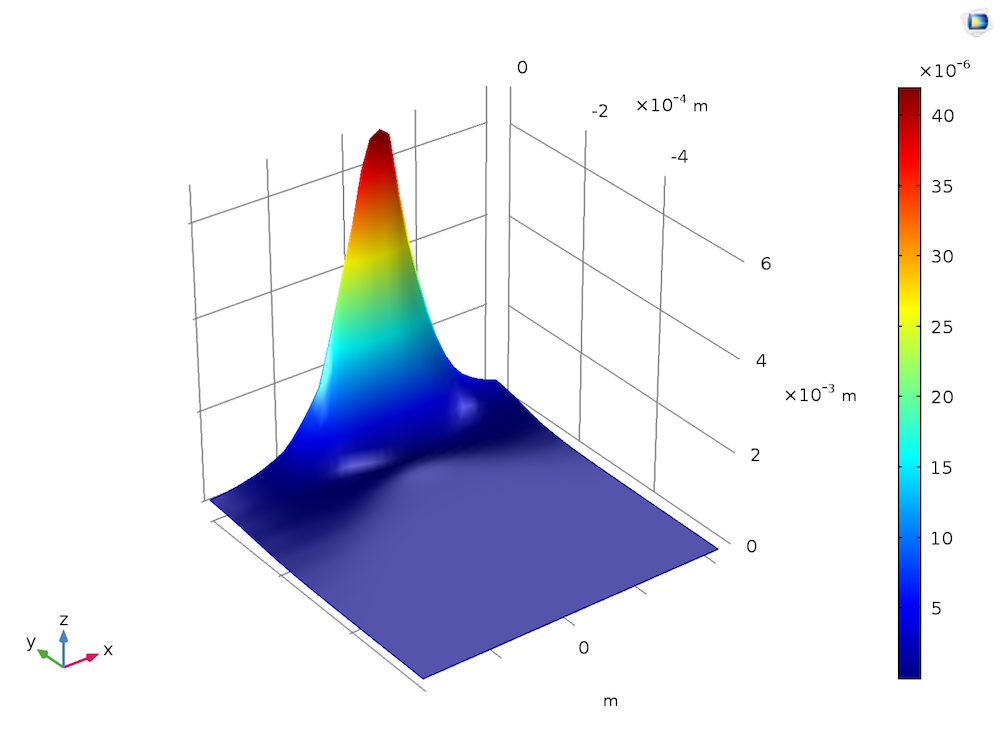
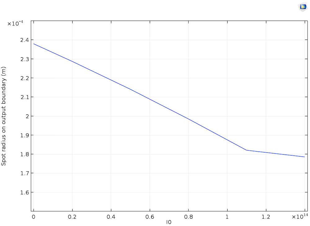
Left: The induced refractive index change, γI, for a high peak intensity, I0 = 14 GW/cm2. Right: The spot radius at the end of the propagation domain versus the peak intensity.
Materials with Electro-Optic Effects
There are materials where the refractive index of the medium can be a function of the applied external electric field, as described in the introduction of this blog post. This applied electric field can be from the DC potential or a slowly varying harmonic potential applied through the coils or contact pads attached to the material. The refractive index optical material property is considered from here on instead of the susceptibility χ.
Mathematically, the refractive index can be represented as a Taylor series expansion of the applied E-field.
For electro-optic materials, the refractive index translates to the following:
where n is the refractive index of the material with no applied E-field, while d1 and d2 are the electro-optic coefficients.
About the Pockels Effect
Crystals such as KDP, lithium niobate (LiNbO3), and cadmium telluride (CdTe) have a refractive index with the dominant first and second terms above. Such media are known as Pockels media, where d1 is known as the linear optic coefficient because the refractive index is a linear function of the electric field.
In COMSOL Multiphysics, the Pockels effect has been demonstrated using an optical modulator. In this model, light propagates through a single silicon waveguide that branches out into two waveguides. Contact pads are applied to the upper branch and excited with a DC voltage, as shown in the image below. This branch of the waveguide can also be defined as a Pockels medium with d1 = 30e-12 m/V.
When no voltage is applied to the contact pads, the light flows unimpeded through both the upper and lower branches and interferes constructively at the point where the branches merge together. However, when a certain voltage is applied to the contact pads, a local electric field is created in the region within the contact pads. The material property in the region under the influence of an external electric field modifies the refractive index of this medium, effectively changing the speed of the light propagating through the upper waveguide. When the light propagating in these upper and lower branches interferes at the location where the branches merge, it leads to destructive interference, with no light propagating forward.
The potential application of the Pockels effect lies in designing optical switches; for example, in the field of photonic integrated circuits. In a tutorial model, we demonstrate a particular kind of optical switching element known as a Mach-Zehnder optical modulator.
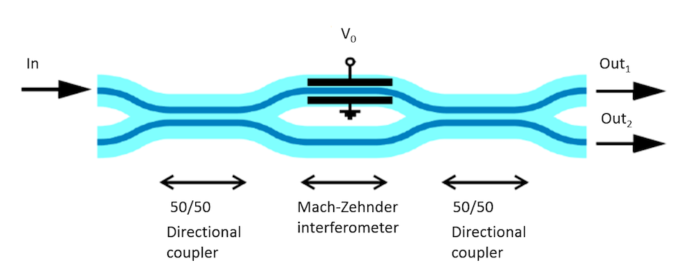
Schematic of the Mach-Zehnder optical modulator.
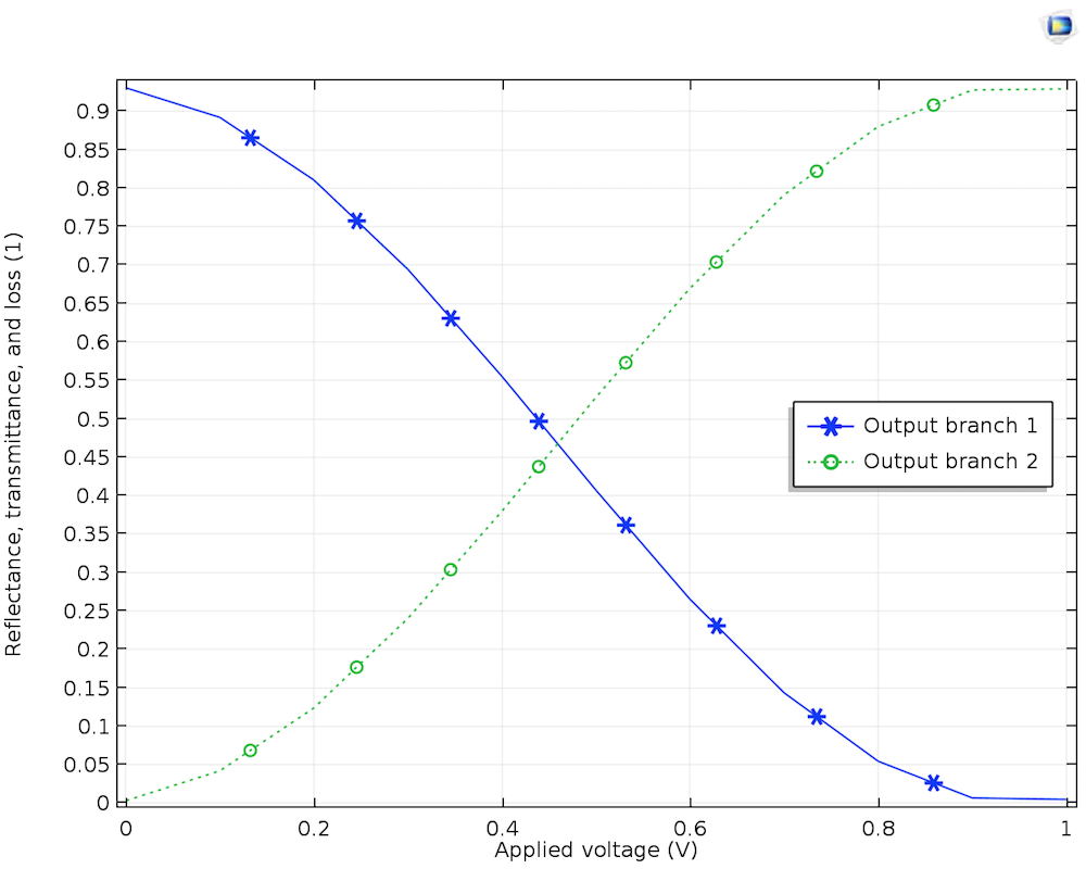
Transmission of the upper output branch 1 and lower output branch 2 versus the applied DC voltage.
About the Kerr Effect
There are certain gases, liquids, and crystals that exhibit a centrosymmetric property, where the first and third term of the Taylor expansion are dominant. In such cases, the refractive index can be defined as a quadratic function of the applied E-field as follows:
Concluding Thoughts on Modeling Linear and Nonlinear Optics
Here, we have discussed different optical materials such as KDP, BK-7, LiNbO3, CdTe, and silicon under an external electric field. These materials show different linear and nonlinear phenomena, such as SHG, self-focusing, and linear and quadratic electric field effects. We have also dealt with the applications of these materials in the laser engineering field, filter design, and optical switches.
Next Steps
Try the tutorials featured in this blog post:
- Plasmonic Waveguide Filter
- Second Harmonic Generation of a Gaussian Beam (Wave Optics)
- Second Harmonic Generation
- Self-Focusing
- Mach-Zehnder Modulator
References
- J. Leuthold, C. Koos, and W. Freude, “Nonlinear silicon photonics”, NaturePhotonics, vol. 4, pp. 535–544, 2010.
- Z. Han, E. Forsberg, and S. He, “Surface Plasmon Bragg Gratings Formed in Metal-Insulator-Metal Waveguides,” IEEE Photonics Technology Letters, vol. 19, no. 2, pp. 91–93, Jan. 15, 2007.
- B. E. A. Saleh and M. C. Teich, Fundamentals of Photonics, John Wiley & Sons, Inc.
- P. B. Johnson and R. W. Christy, “Optical constants of the noble metals,” Phys. Rev. B, vol. 6, no. 12, pp. 4370–4379, Dec. 15, 1972.
- Y. R. Shen, The Principles of Nonlinear Optics, John Wiley & Sons, Inc.

Comments (7)
Eloise Passos
February 22, 2019How I can simulate the photorefractive effect in COMSOL?
Uttam Pal
March 5, 2019Dear Eloise,
You would be interested to go through the “Single-Bit Hologram” and “Holographic Page Data Storage Simulation” model, which talks in detail about the modulation of the refractive index.
Single-Bit Hologram: https://www.comsol.com/model/34921
Simulating Holographic Data Storage in COMSOL Multiphysics blog: https://www.comsol.ch/blogs/simulating-holographic-data-storage-in-comsol-multiphysics
Alex Mak
July 20, 2019Do you have instructions for simulations stimulated raman scatter or coherent anti-stokes raman scatter?
Uttam Pal
July 24, 2019Dear Alex,
We don’t have exact example models for Stimulated Raman scattering and Anti-Stokes Raman Scattering effects. However you can do a literature survey, papers are available. Most relevant example to start would be “Scatterer on Substrate” https://www.comsol.com/model/14699 , which discusses the scattering and absorption cross-sections.
Fariza Suhailin
December 31, 2019Is there any example of plasmonic mode excitation using fiber optic?
Uttam Pal
January 2, 2020 COMSOL EmployeeDear Fariza,
I would recommend you to write to support@comsol.com, so we can discuss it further.
NAGARAJAN N
August 24, 2021Dear Pal,
Can I use electro optic coefficient in Semiconductor module? like how you will demonstrate MZI Interferometer? In the core refractive index –ncore-0.5*ncore^3*r13*es.EY are used for voltage tuning. Like this, i would like add electro optic coefficient in semiconductor module. if i add ncore-0.5*ncore^3*r13*semi.EY its showing error.