

A COMSOL Multiphysics® simulation typically includes one or more field quantities in its output. Depending on the number of field quantities, the geometry’s complexity, and the mesh density required for valid results, simulations can include millions of degrees of freedom (DOFs). Oftentimes, storing one or more scalar quantities or the results on a small geometry part is sufficient. Here, we explore tools for storing selected output quantities and minimizing model file sizes and the time required to display this data.
Two Options for Storing Relevant Simulation Output
COMSOL Multiphysics provides two ways for you to include only selected parts of a solution in your output. The first option is to define one or more selections, including the points, boundaries, or domains of interest, so you can restrict the output from the study to only include the fields in the parts of the geometry that those selections define. This method is straightforward and suitable if you are only interested in the simulation output within a certain part of the geometry, where you can perform postprocessing and access the fields and derived quantities as usual.
Note that if you store the solution for some boundaries or points, only the solution fields (the dependent variables) are available using this method. This means that derivatives and quantities that include derivatives, such as stresses and fluxes, are not available as they require that the solution is also available in the domain. If you are interested in storing some derived values such as stresses on just a few boundaries or points of interest, you will want to use our second option.
The second option is to add an ODE and DAE interface to define a new dependent variable, to which you can transfer the quantity of interest. The quantity of interest could be a global scalar quantity, such as the average or maximum of some field, or it could be the field value along some boundary. (In the latter case, using a selection provides an easier way of achieving the same result.) This method is useful in situations where the output of interest is a global scalar value that you transfer to a single degree of freedom as a variable within a simple algebraic equation. As mentioned above, it is also useful if the quantity of interest is a derived value based on derivatives, such as stresses and fluxes.
Creating a Selection to Store Selected Parts of a Solution
To only store the solution in a selected part of a geometry, create a named selection in the model component. To do so, right-click Definitions and choose a selection from the Selections submenu. An Explicit selection is simple to use if you want the selection to include some specific geometric entities — for example, domains, boundaries, or points. You can give the selection node a descriptive label like Surrounding Air or Substrate Contact. You can use several selection nodes to represent different parts of the geometry and combine them, either when determining what to store in the output or by creating another selection node that implements a Boolean operation, such as a Union or an Intersection selection node. Use one or more of these created selections in the study step settings to define the parts of the geometry for which the solution will be stored.
Example: A Selection for Storing the Deflection on the Top Surfaces of a Mechanical Design
In a solid mechanics simulation, the value of the deflection (displacement) on one or more specific surfaces or points of interest can provide valuable information, which may be sufficient for you as the output from a simulation. The following plot, for instance, indicates the selected top surfaces on the model geometry for a feeder clamp within the Graphics window.
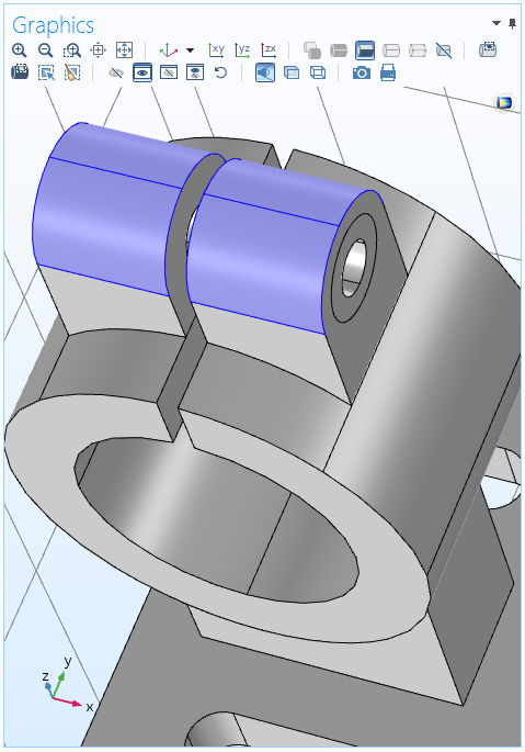
Selected surfaces for a solid mechanics simulation.
To store only the solution on those surfaces (boundaries), create an Explicit selection with the input entities set to the four top surfaces within the geometry where you want to store the solution. If a surface or point is not part of the created geometry, you can add extra Curve or Point nodes in the geometry sequence to divide a boundary or add a point (and a mesh node) at the desired location. The settings for the Explicit selection node appear as shown below.
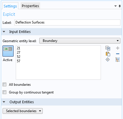
Explicit selection node settings.
Here, the label has been changed to Deflection Surfaces to reflect what the selection contains.
You can now modify what to store in the output. In the Settings window of the Study step node, locate and expand the Values of Dependent Variables section. This section contains Store fields in output settings, where you can choose For selections from the drop-down menu. You can then click the Add button to open a list with available selections. In this case, choose the Deflection Surface selection and click OK.
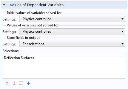
Settings for storing the deflection for the selected surfaces in the geometry.
Now you can run your simulation. The only output will be the solution on the top surfaces, which you can visualize using a Surface plot.
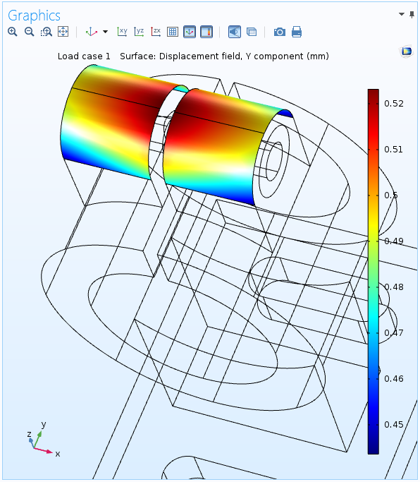
The displacement in the y direction on the selected surfaces in the geometry. For the rest of the geometry, there is no solution output.
For the solution at points, you can postprocess the output using a Point Evaluation node under Derived Values and display the total displacement, for example. You can also use a Point Graph node in a 1D Plot Group to plot the displacement versus time in a time-dependent simulation or a parameter value in a parametric sweep.
Creating a Variable of Interest to Store in the Output
If you are interested in a scalar quantity, you only need a single degree of freedom (variable) that represents that quantity in the output. You can create such a variable as a simple algebraic equation using a global equation defined via the Global ODEs and DAEs interface. This interface and similar physics interfaces for defining ODEs and DAEs on domains or at points, for instance, are available under Mathematics > ODE and DAE Interfaces in the Add Physics window and in the Model Wizard. In the Settings window for the Global Equations node, define the name of the variable and the simple equation that sets it to the scalar quantity that you want to include in your simulation output.
Scalar coupling operators are important features in COMSOL Multiphysics to utilize for this purpose as well. With these powerful tools, you have the ability to create scalar quantities that are made globally available within the model.
Example: A Variable that Represents the Average Temperature
Say that you are primarily interested in the average temperature within the model geometry. To extract its value, add an Average Coupling Operator (aveop1, for example), defining it to be valid in the entire geometry (all domains) or in the domains of interest. You can then use this operator in a global algebraic equation to make it available in the simulation output as a scalar variable. If you want to store the maximum temperature instead, you can use a Maximum Coupling Operator.
The equation that the Global ODEs and DAEs interface solves for is
In this case, however, the equation should only set the variable equal to the average temperature. As such, it is sufficient to enter aveop1(T)-avtemp if you have called the variable in the algebraic equation avtemp. Remember that the Global ODEs and DAEs interface sets the expression to zero to form the equation, thus solving the simple equation avtemp = aveop1(T). Here, T represents the temperature field in the geometry, which is the dependent variable that you solve for but don’t want to include in the output. The following screenshot shows the Settings window for a Global Equations node in the Global ODEs and DAEs interface for this case.
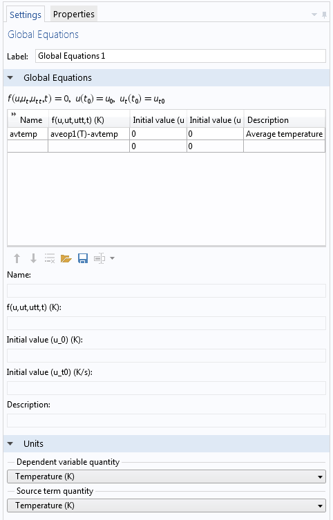
Global Equations node settings for creating a variable to store.
Notice the Units section within the Settings window shown above. To avoid unit inconsistencies and to evaluate the created variable with the correct units, you should adjust the respective units for the dependent variable and for the source term.
Your final step is to set up the simulation so just the new scalar variable that you have defined is stored in the output. The following plot shows the average temperature in a geometry for a time-dependent simulation as a Global plot defined in a 1D Plot Group.
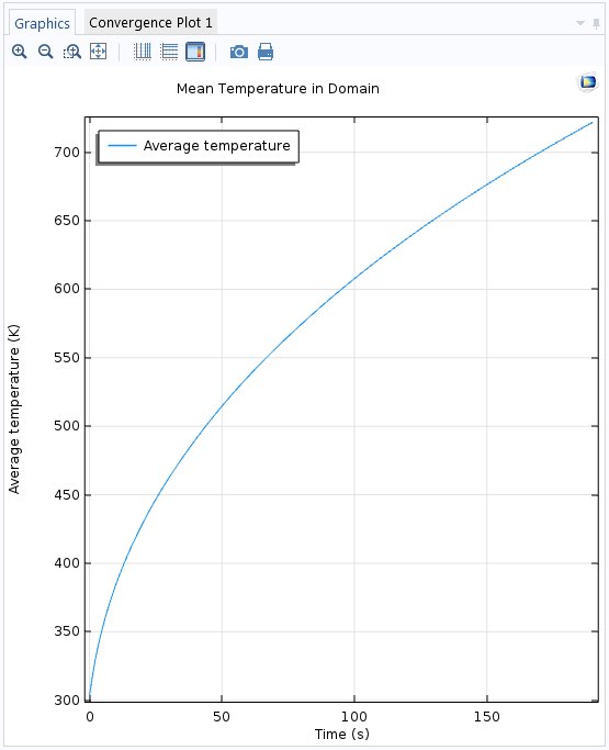
The mean (average) temperature versus time, computed as a single scalar output from a time-dependent simulation.
Controlling What Is Stored in the Output
In the study that you want to perform, first make sure that you have access to the solver configurations by right-clicking the main Study node and choosing Show Default Solver. Select Solver Configurations > Solution > Dependent Variable to access the settings for the dependent variables. In the cases above, there will be two nodes: a Field node (temperature) and a State node (average temperature). The first node represents the full temperature field in the geometry, while the second node represents the variable for the average temperature.
Click the Temperature node to display its Settings window. At the bottom of the General section, clear the Store in output check box so that the solver no longer stores the temperature field in the output.
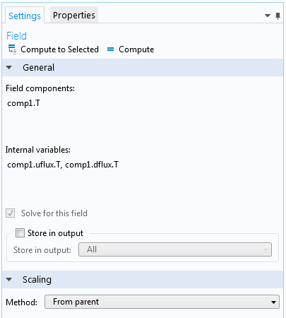
Clearing the Store in output check box within the Temperature node settings.
When you have computed the solution, the scalar quantity will be available as a variable that you can display in a table using a Global Evaluation node. You can also plot a Global graph plot to show the deflection versus time or the mean temperature versus some parametric solutions. Since there are no field solutions, any plots that show such variables, or quantities using such variables, will appear with values of zero.
Example: An Algebraic Equation for the Equivalent Stress on the Top Surfaces
Let’s revisit our feeder clamp model to show how to use an algebraic equation to store the equivalent stress (von Mises stress) values on the top surfaces. To do so, add a Boundary ODEs and DAEs interface, available under Mathematics > ODE and DAE Interfaces in the Add Physics window and in the Model Wizard.
In the Settings window for the main Boundary ODEs and DAEs interface, use the same Deflection Boundaries selection for the top surfaces. Make sure to specify the units so that they are compatible with a stress quantity. You can do so by choosing Stress tensor as the quantity for the new dependent variable and for the source, which is the von Mises stress from the main Solid Mechanics interface.
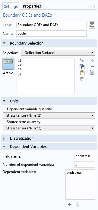
The settings for the Boundary ODEs and DAEs interface, set up for a mechanical stress quantity.
In the Distributed ODE subnode, you define the algebraic equation that sets the new dependent variable bndstress (defined on the top surfaces only) equal to the predefined variable for the von Mises stress, solid.mises, from the Solid Mechanics interface: bndstress-nojac(solid.mises).
The nojac() operator is required, since we do not want this equation to contribute to the Jacobian (the system matrix) for the full model. You enter this expression in the source term and set all other coefficients to zero to solve the equation 0 = bndstress-nojac(solid.mises) (that is, bndstress = nojac(solid.mises)).
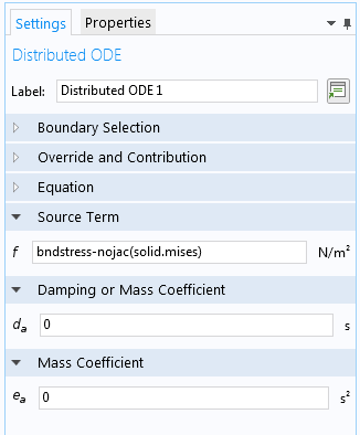
The settings in the Distributed ODE node for defining an algebraic equation for the boundary stress.
Before solving, you have to clear the Store in output check box in the Displacement field node under Dependent Variables in the solver sequence. You can then compute the solution and only store the stress values on the top surfaces, which you can plot using a Surface plot.
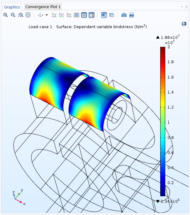
A plot of the von Mises stress, stored only for the top surfaces.
Optimize Your Simulations with Storing Solution Techniques
As we have shown here today, with just a few simple steps, you can set up a simulation where only part of the fields computed for, or even just one or a few scalar quantities of interest, can be stored in the output. These modeling techniques can significantly reduce your model file size and the time it takes to calculate and display these scalar quantities of interest. This is especially true if you plan to make simulations that include large parametric sweeps or long, detailed time-dependent studies.
To learn about other tools in COMSOL Multiphysics that are designed to optimize your simulation workflow, browse other posts within our General category on the COMSOL Blog. If you have further questions relating to the modeling techniques presented here, please feel free to contact us.

Comments (11)
Andrii Lesiuk
September 3, 2016Hi. Is this option available only in version 5.2 or in earlier version 5.1 as well? I mean the method with Selections.
Magnus Ringh
September 5, 2016Hi Andrii, yes, the method with Selections in available from version 5.2. If you want to upgrade to the latest version of COMSOL Multiphysics (version 5.2a), please contact your local COMSOL representative.
Zhichao Jia
September 5, 2016Good work!!!
Tarkes Dora
March 12, 2017Can anyone suggest how to store all the eigenfrequencies/values ?
Magnus Ringh
March 13, 2017Hi Tarkes, to store all eigenfrequencies or eigenvalues but not the corresponding field solutions, solve the eigenmode problem but clear the “Store in output” check box for the dependent values. You can then export the eigenfrequencies or eigenvalues (stored in the built-in variables “freq” and “lambda”, respectively).
Mahmoud Elzouka
May 29, 2017Thank you for the article,
I have a quite relevant question:
How can I remove the solutions corresponding to certain eigenvalues?
Thanks
Sergey Yankin
December 21, 2022 COMSOL EmployeeHi Mahmoud, you can use Remove Solution feature: https://www.comsol.com/support/knowledgebase/1255
Wen Luo
December 13, 2023Hi,
Thanks! Nice article. Yet I have one question regarding using the ODE
in Example: A Variable that Represents the Average Temperature
We already use Average Coupling Operator to calculate the average temperature over the domain, (which, in my view, will give us the average temperature), but why we still need an ODE interface, to solve simply “avtemp = aveop1(T)”? Is it to store the output from Average Coupling Operator? Can we use Probes to store the output from Average Coupling Operator and visualise the results via Probe Table Graph?
Magnus Ringh
December 14, 2023 COMSOL EmployeeHi Wen, thanks for your feedback.
Using an separate ODE (which is computationally “cheap” because it only adds a single degree of freedom) and storing it in the output makes sure that the data is available after solving. While a probe does capture the same data, its values will be empty (0) if you then want to reevaluate it after computing the solution without storing the temperature field, for example.
Best regards,
Magnus
Wen Luo
December 21, 2023Hi Magnus,
thanks for the reply.
What if we store the output for the probe? As you said in the article, Study 1 –> Solver Configurations –> Solution 1(sol1) –> Dependent Variables 1 –> Temperatures, in the Settings, we can click “store in output” for “selection”. In this case, will the data be stored? It seems in my results, even though I do this, the probe table graph cannot show any data…
thanks,
WEN
Magnus Ringh
December 21, 2023 COMSOL EmployeeHi Wen,
Yes, there will be a Probe Solution dataset, which you can use to plot or evaluate the probe data for the probe that you have defined after computing the solution.
Best regards,
Magnus