Problem Description
I am solving a time-dependent wave-type problem, what mesh and solver settings should I adjust for better accuracy and runtimes?
Solution
The accuracy of a time-dependent model solving for electromagnetic, acoustic, structural, or any other kind of wave-type model is limited by how well the finite element mesh resolves the waves in space and by how well the time steps resolve the temporal variations. This article describes how to control the mesh and the solver settings for such problems.
Note: If you are solving a model using a Time Explicit formulation, such as the Pressure Acoustics, Time Explicit; Elastic Waves, Time Explicit, Convected Wave Equation, Time Explicit; or the Electromagnetic Waves, Time Explicit physics interfaces, this knowledgebase entry does not apply. Please refer to the documentation for advice on mesh and solver settings when using these interfaces.
Before starting your modeling, you should know two things. First, the maximum frequency content of your excitation. Define this as a Global Parameter, for example: f_max. Second, the material properties in all domains. This information governs what size mesh you will need in all domains, since the material properties govern the shortest possible wavelength. If there are any material or boundary condition nonlinearities, consider that these may lead to frequency doubling or other phenomena that may lead to much higher frequency content. If you anticipate any step changes in the loads or boundary conditions, first read: Knowledge Base 1244: Solving Wave-Type Problems with Step Changes in the Loads
Once you know the maximum frequencies that you expect to model, and the material properties, you can build and mesh your model. By default, second order (quadratic) elements are used in the electromagnetic, acoustic, and structural transient interfaces. At a bare minimum, the mesh must fulfill the Nyquist criterion, so at least two elements per local wavelength in each domain. However, this will usually be of unacceptably low accuracy. Practically speaking, at least five second order elements per local wavelength should be used, but very rarely more than ten elements per wavelength. Set up a User-controlled mesh with different Size features applied to the different material domains. The Free Triangular (in 2D models) and Free Tetrahedral (for 3D models) meshes are preferred, but the other element types (Hexahedral, Triangular Prisms, and Pyramids) can be used if there are high aspect ratio structures, thin layers, material anisotropy, or other reasons to expect strong variations in the solution in only one or two directions. PMLs, which are supported by the Pressure Acoustics, Transient interface, should use mapped or swept elements. Also define a Global Parameter (for example: N) to control the number of elements per local wavelength and a set of Variables to define the local wavelengths in different domains, as demonstrated in the screenshot below.
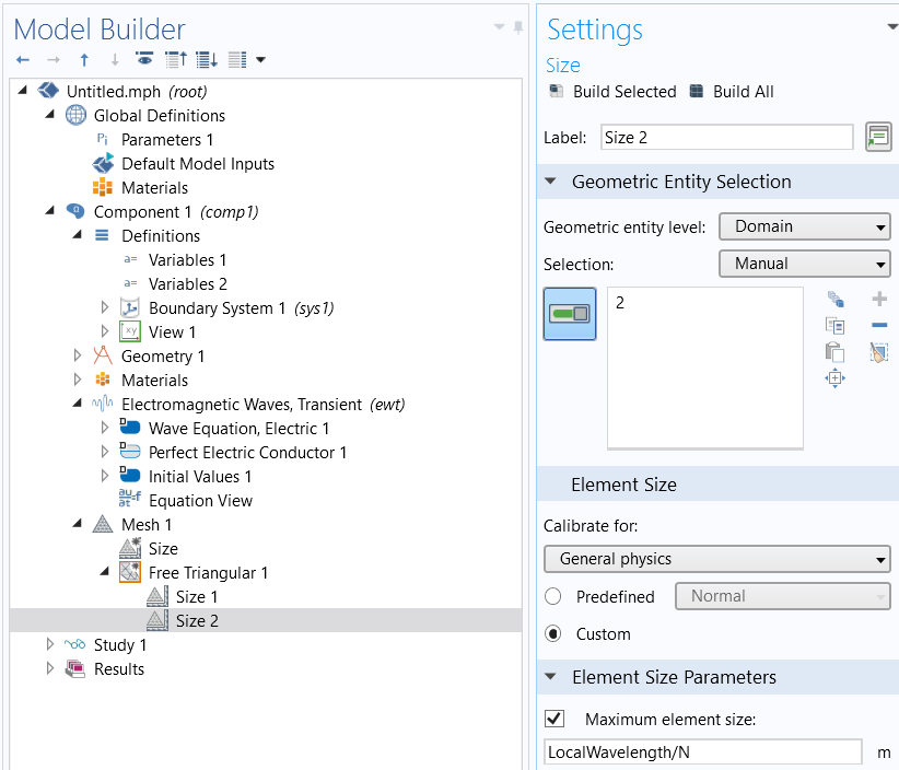
Manually setting the element sizes
Bear in mind that in structural mechanics, different types of waves have different wavelengths. In a bulk material, shear waves typically have shorter wavelengths than pressure waves. However, in for example a thin part of the geometry, bending waves can be even shorter. As you cannot always tell the exact wavelength in advance, be sure to inspect the solution - does it look smooth and well resolved? - and consider running a mesh convergence study if in doubt.
For most interfaces, with the transient Pressure Acoustics, Thermoviscous Acoustics, and Aeroacoustics interfaces as notable exceptions, the Time-Dependent Solver will per default continuously adjust the time step in order to fulfill your specified tolerances. The Relative tolerance field in the Time Dependent settings (shown below) controls how the solver will adjust the time step. Smaller numbers will lead to smaller time steps and higher accuracy. Note that changing the number of output Times in the Time Dependent node controls only the output times, but has little effect on the time steps actually taken by the solver.
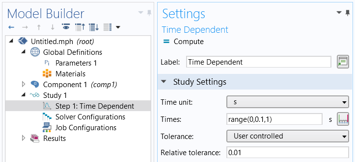
The output time steps and relative tolerance settings
However, since you already know your maximum local mesh size and maximum frequency, it is more computationally efficient to manually set the timestep. The time step should resolve the wave equally well in time as the mesh does in space. Longer time steps will not make optimal use of the mesh, and any shorter time steps will lead to longer solution times with no considerable improvements to the results. The relationship between wavespeed, c, maximum mesh size, h, and time step length, Δt, is known as the CFL number:
CFL = cΔt/h
We have already manually defined the maximum mesh size to be 1/N of the local wavelength (as described above), so this can re-written in terms of the frequency f, and N the number of elements per local wavelength:
CFL = fNΔt
or, rearranging:
Δt = CFL/Nf
With the default second order, quadratic, mesh elements, the CFL number should be less that 0.2, and a value of 0.1 proves to be near optimal, it is helpful to define this CFL number as a Global Parameter as well.
For the aforementioned acoustics interfaces, the time-dependent solver is per default already set up for manual time stepping, and with the CFL number in mind. In order for it to take a suitable time step, enter your defined fmax for the Maximum frequency to resolve, on the Setting tab of the physics interface node. This will generate a manual time step 1/(60*fmax), which if you mesh with 6 elements per wavelength corresponds to a CFL number of 0.1.
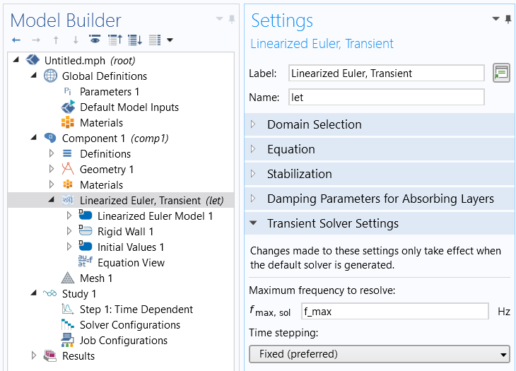 Setting the maximum frequency to resolve in the transient acoustics interfaces
For other interfaces, implement the manual time-step size in the Time-Dependent Solver settings, usually found at Study > Solver Configurations > Solution > Time-Dependent Solver, Time Stepping settings. (If these settings are not already in the Study branch, then right-click on Study and select Show Default Solver.) Set the Time Stepping Method: to Generalized alpha, set the Steps taken by solver: to Manual and set the Time Step to:
CFL/(N*f_max)
The Generalized alpha solver is preferred for the reasons outlined in: Knowledge Base 1062: BDF, Generalized Alpha, and Runge-Kutta Methods
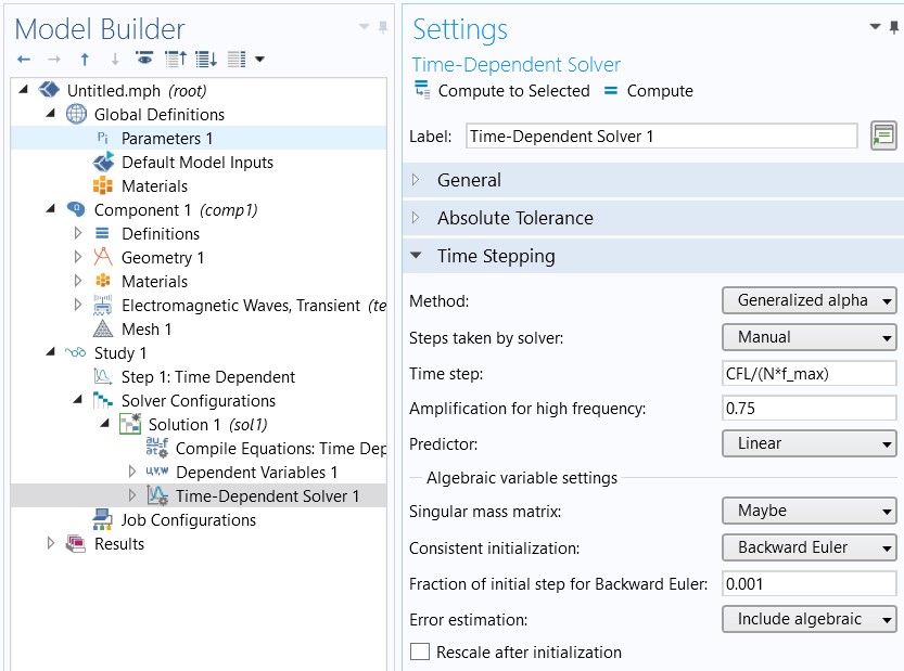
Manually setting the time-step size
For an example of these mesh and solver settings, see the Gaussian Explosion in the Application Library of the Acoustics Module.
For an example of modeling a nonlinear material within the RF Module, see the Second Harmonic Generation of a Gaussian Beam. The same example is also available within the Wave Optics Module: Second Harmonic Generation of a Gaussian Beam
See also:
Knowledge Base 1244: Solving Wave-Type Problems with Step Changes in the Loads
Knowledge Base 1240: Manually Setting the Scaling of Variables
COMSOL makes every reasonable effort to verify the information you view on this page. Resources and documents are provided for your information only, and COMSOL makes no explicit or implied claims to their validity. COMSOL does not assume any legal liability for the accuracy of the data disclosed. Any trademarks referenced in this document are the property of their respective owners. Consult your product manuals for complete trademark details.