Problem Description
How do I gain confidence in the accuracy of the solution to my problem? How do I perform a mesh refinement study?
Solution
All of the numerical methods used within COMSOL Multiphysics® discretize the modeling space via a Mesh that serves two purposes. First, this mesh is used to approximate the CAD geometry. Second, the approximate solution to the problem is solved at discrete points in space defined by this mesh. As this mesh is refined, the solution will tend to more accurately approximate the true to solution to the boundary value problem being posed. ( Not all physics problems within COMSOL are boundary value problems, in particular the governing equations solved by the Ray Optics and Particle Tracing interfaces are ordinary differential equations. Even these, however, still require a discretization of the CAD geometry. )
To gain confidence in the accuracy of your model, you must re-solve the model on progressively finer meshes and compare results. In the limit of mesh refinement, well-posed problems will be convergent. In practice, there is a limit to how much mesh refinement can be done before you exceed the computational resources that you have available. (See also: Knowledgebase 1030: Error: "Out of memory". )
There are several different strategies that you can take to performing a mesh refinement study:
Adaptive Mesh Refinement
When using adaptive mesh refinement, as shown in the screenshot below, the software will compute the solution on an initial mesh and estimate where the error is high. The geometry will then be re-meshed with finer elements in these regions and the model re-solved on this new mesh. This feature allows you to control how many levels of adaptive mesh refinement are performed, how many elements will be created on the finer mesh, what metric to use to estimate the error, as well as the method used to adapt the mesh. This functionality is not available in combination with all physics interfaces, Ray Optics and Particle Tracing for example.
Example models from the core COMSOL Multiphysics package that demonstrate the usage of this functionality include Implementing a Point Source and Stresses in a Pulley.
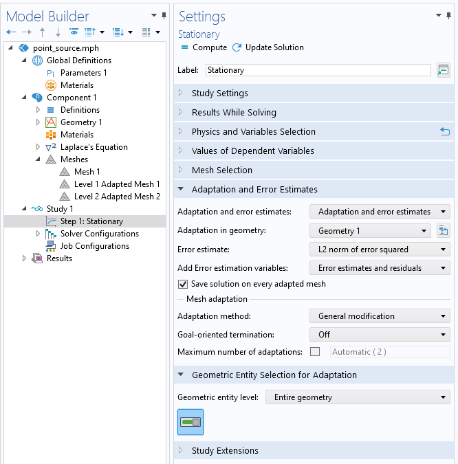
Screenshot showing the adaptive mesh refinement settings for a stationary study, the created meshes, and the data set containing the results on different meshes.
The results of adaptive mesh refinement will be a set of different Meshes, viewable within the Mesh branch, and a single Data Set that combines the results from all the levels of mesh refinement. The initial mesh that you start with can be either manually set up, or using the software default mesh.
The settings and interface for adaptive mesh refinement of a time dependent study look a little bit different, as shown in the screenshot below. Rather than just a single mesh, several meshes will be created during the simulation time-span.
![]()
Screenshot showing the adaptive mesh refinement settings for a transient study. Several meshes corresponding to different times are created, and stored within a single data set.
Manually Defining Mesh Refinement
When using this approach, you will need to manually edit the meshing sequence and use a combination of different settings to define different mesh sizes in different parts of the model. See the Basics of Meshing tutorial from the COMSOL Learning Center. A simple introductory application example on using meshing sequences is: Using Meshing Sequences.
The advantage of this approach is that you can more directly control how fine of a mesh is created, and you can also control the aspect ratio of the elements created. This is particularly advantageous if you know that the solution will vary strongly, or gradually, in one or two directions. This approach does require a greater level of interactivity, effort, and understanding as compared to adaptive mesh refinement, but it can lead to a strategy that uses less computational resources.
Introduce a parameter that controls the mesh size and use a Parametric Sweep to sweep over a range of values that control the mesh. To learn how to set up a parametric sweep, see: Performing a Parametric Sweep Study in COMSOL Multiphysics®. The results will be available within a single Data Set that contains all the parametric solutions.
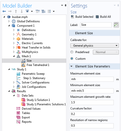
Screenshot showing a manual meshing strategy, along with the Parametric Sweep feature and the resultant Data Set.
An example model from the core COMSOL Multiphysics package that demonstrate the usage of this functionality is The Blasius Boundary Layer. Another example, that uses the Structural Mechanics Module, is Stress Analysis of an Elliptic Membrane.
Using Physics-Controlled Mesh settings
It is also possible to use the default Physics-controlled mesh settings. Depending upon the physics involved in the model, the software will adjust the mesh based upon the geometry, and possibly also the applied domain and boundary conditions within the physics as well as the materials properties. The latter only occurs for electromagnetic waves problems, as demonstrated here Automated Meshing for Electromagnetic Waves, Frequency Domain Simulations.
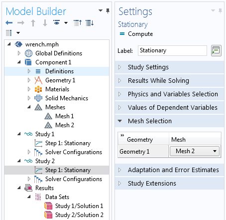
Once different meshes have been created, they can be selected within the settings for each Study Step.
When using this approach, you have no direct control over the mesh, but it is very easy to use. Create several different meshes, each with their own Element Size: setting and introduce several different studies. Select the mesh as shown in the screenshot above. The results will be contained in different data sets, one for each study.
Increasing Element Order
In additional to the above techniques it is also possible, albeit less common, to study the effect of changing element. See: Understanding, and changing, the element order. Each physics interface defines an element order for approximating the fields within each element. This can be increased or decreased via the Discretization settings as shown in the screenshot below. Increasing discretization significantly increases memory usage. Use caution when altering this setting for multiphysics models, especially when mixing element orders in different physics. See also: Keeping Track of Element Order in Multiphysics Models.
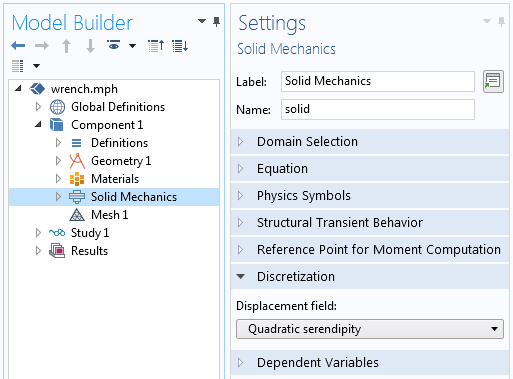
The discretization setting for a physics.
General Remarks
These approaches all presume that the software will converge to a solution for every different mesh. This is not necessarily the case for nonlinear problems, which may not converge if the mesh is too coarse. Other strategies for dealing with nonlinear models as addressed here: Improving Convergence of Nonlinear Stationary Models.
Comparing and Evaluating Results
Once you have used any one of, or any combination of, the above approaches you will want to compare the results between different cases. To view the differences between any two cases, create and use a Join data set within Results > Data Sets. Adjust the settings for the two sets of data that you wish to compare and select the Combination method to be Difference to create a set of data the is the difference between two different levels of mesh refinement, as shown in the screenshot below.
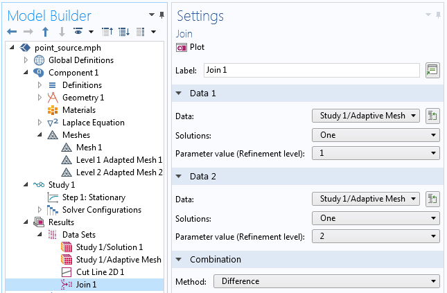
The Join data set can evaluate the difference between solutions.
Be careful in evaluating the results of a mesh refinement study. Depending upon what metric you are evaluating, some quantities will converge faster, or slower, than others. Generally speaking integrals over the entire model will converge the most quickly, and local values the most slowly with mesh refinement. Also be careful in evaluating the derivatives of the fields at sharp corners, these will be locally non-convergent although they will not affect much the overall accuracy of the model far away from the singularity. For more details, see:
Singularities in Finite Element Models: Dealing with Red Spots
How to Identify and Resolve Singularities in the Model when Meshing
Should I Fillet the Geometry in My Electromagnetic Heating Analysis?
Additional Resources
The following articles address specific cases but are also of general interest:
COMSOL makes every reasonable effort to verify the information you view on this page. Resources and documents are provided for your information only, and COMSOL makes no explicit or implied claims to their validity. COMSOL does not assume any legal liability for the accuracy of the data disclosed. Any trademarks referenced in this document are the property of their respective owners. Consult your product manuals for complete trademark details.