Understanding and Changing the Element Order
In the settings for a physics interface node in COMSOL Multiphysics®, there is a Discretization section where you can see the element order being used. You have the option of changing this setting. Here, we discuss both the meaning and significance of the element order and discretization for a simulation, how you can change the settings for it, and what effect this has on the mesh and solution for your model.
What Is the Meaning of Element Order and Discretization?
Most physics interfaces within COMSOL Multiphysics® use the finite element method to solve the underlying partial differential equations. The finite element method works by discretizing the modeling domains into smaller, simpler domains called elements. The solution is computed by assembling and solving a set of equations over all of the elements of the model. The solution to these equations approximates the true solution to the partial differential equation.
The equations within each element are also known as shape functions and can be of different order. For example, in the simplest case of a one-dimensional finite element model, the shape functions within each element are simply a set of polynomials defined over the domain. In the image below, the set of linear (first-order), quadratic (second-order), and cubic (third-order) shape functions are plotted. The solution within the elements is based upon a linear sum of these shape functions.
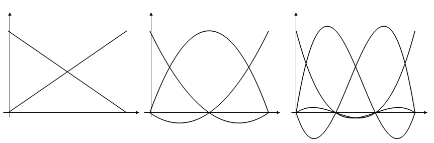
Plots of linear (left), quadratic (center), and cubic (right) shape functions within a one-dimensional element.
Different physics interfaces can use different sets of shape functions. That is, each physics interface has its own unique discretization settings that govern what order shape functions are using for those dependent variables, as shown in the example screenshot below for the Electric Currents physics interface.
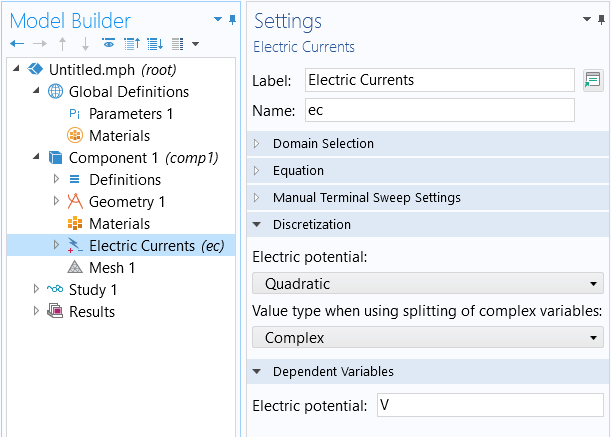
The discretization settings for a physics interface.
The default discretization in many cases is second order (quadratic), and this is partially because many of the partial differential equations have a dominant second derivative term. Problems involving fluid flow and transport are generally by default using a first-order, linear discretization. Based upon the particular modeling situation, changing the discretization may be motivated, and it is possible to change the discretization for each different physics interface independently, but doing so has several consequences.
Lowering the discretization without changing the number of elements will lead to a model that requires less computational resources but will have lower accuracy. Increasing the discretization without changing the number of elements will lead to a more accurate solution, but will require greater computational resources. Note that increasing the element order is one approach to validating your model, but that you will likely want to study refining the mesh instead by performing a mesh refinement study.
There are sometimes additionally the options of Lagrange and serendipity elements for the quadratic and higher discretizations. This setting has an effect only if rectangular, prismatic, pyramidal, or hexahedral elements are present in the mesh. The Lagrange element introduces additional nodes (degrees of freedom) within the elements as visualized in the figure below. Although the serendipity element has fewer nodes per element, it often exhibits quite good accuracy for the same mesh but a lower computational cost compared to the Lagrange element. If a mesh can be created that is dominated by rectangular, prismatic, pyramidal, or hexahedral elements, it is usually worth using the serendipity discretization, if it is available within the physics.
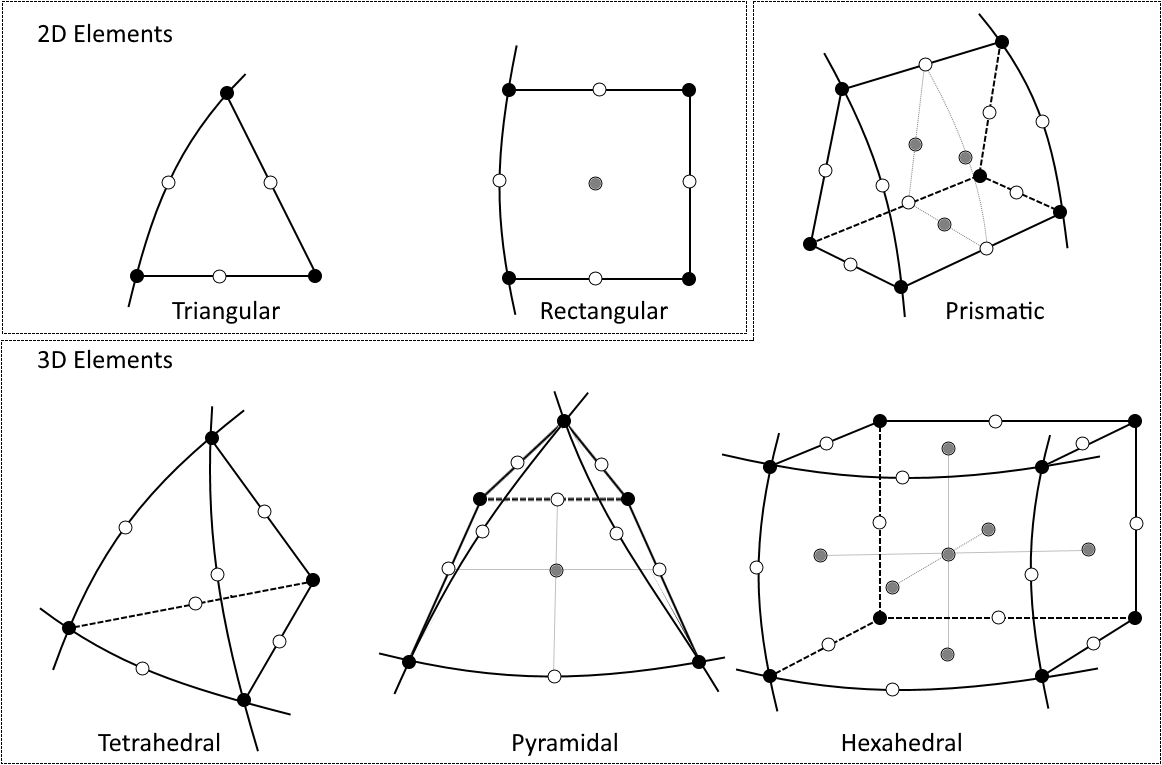
Visualization of node placement in second-order elements. The black, white, and gray nodes are all present in the Lagrangian elements. The gray nodes as removed for the serendipity elements.
Effect On Mesh
When modeling in 2D, 2D axisymmetry, or 3D, the discretization settings within the physics also affect the mesh elements. The mesh elements in 2D and 3D additionally serve the purpose of approximating the true CAD geometry, and they do so by approximating the shape of the boundaries of the model via a set of geometric shape functions that have the same order as the lowest discretization order used in any of the enabled physics interfaces within the model.
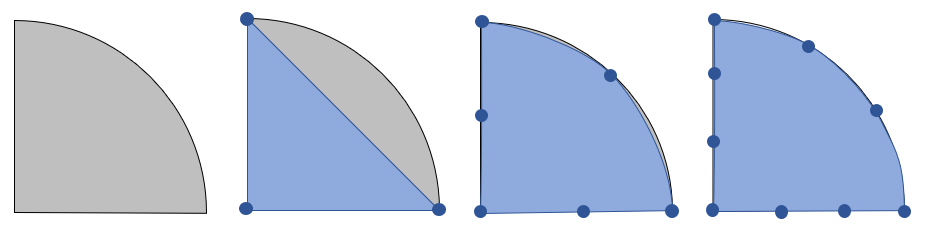
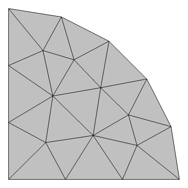
A semicircular domain (left) discretized with linear (center, left), quadratic (center, right), and cubic (right) geometry shape functions. The blue circles represent the nodes.
For example, consider a semicircular domain, as shown above, discretized with the simplest possible mesh consisting of a single triangular element. The straight sides of the modeling domain are precisely represented regardless, but the curved boundary can only be approximately represented by the geometric shape functions. With a linear shape function, this approximation reduces to a triangular element that quite poorly represents the modeling domain. Quadratic and cubic shape functions give a much better representation of the underlying geometry. A consequence of this is that, when linear geometry shape functions are used, you generally need a much finer mesh on curved boundaries just to get an accurate representation of the underlying CAD geometry. A good rule of thumb, when using linear geometry shape functions, is that at least 8 elements are needed per 90° arc to resolve the boundary with less than 1% error. On the other hand, with quadratic and higher-order shape functions, even just two elements per 90° arc are sufficient to be significantly below 1% error in representing the CAD geometry. These rules of thumb are only starting points as to how to create an initial mesh; a mesh refinement study is always called for.
When building and viewing the mesh, the elements will always appear as straight sided, even if the underlying shape functions are of a higher order. Only when results are plotted will the element boundaries be plotted in a way to show the underlying shape function.
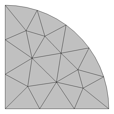
A semicircular domain is meshed using a linear Lagrange (left) and cubic Lagrange (right) geometry shape function. Note the difference in how the curved boundary is represented.
The information about the geometry shape order is also shown near the top of the log that is generated when the model is solved. This log file will look something like:
<---- Compile Equations: Stationary in Study 1/Solution 1 ----------------------


Started at ....


Geometry shape order:
Quadratic


Running on ...
Multiphysics Models and Discretization
When a model includes several different physics, it is possible that one physics will have different discretization settings from the others. The geometry shape order will, by default, be governed by the lowest-order discretization in any of the active physics. An explanation for what discretization is used for some physics and combinations of physics is given below.
Fluid Flow
The default for laminar and turbulent flow problems is a so-called P1+P1 discretization. Linear shape functions are used to solve for both the fluid velocity and the pressure fields. It is possible to raise the discretization to P2+P1, meaning that quadratic shape functions are used for the velocity, but linear basis functions are used for the pressure. Thus, for a model with P2+P1 discretization, the linear geometry shape function is still used.
Fluid–Structure Interaction
When solving for fluid–structure interaction, the P1+P1 discretization is used by default for the fluid problem, but a quadratic discretization is used for the solid mechanics problem. Although these physics are solved on different (nonoverlapping) domains, the same geometry shape order must still be used for all physics.
Please note that although it is possible to manually set the geometry shape order within the General settings for the Component node in the model tree, this should only be done with a thorough theoretical understanding.
For further information on element order, specifically with respect to multiphysics models, see our blog post on keeping track of the element order in multiphysics models.
Submit feedback about this page or contact support here.