Physics, PDEs, Mathematical and Numerical Modeling
The Laws of Physics, Mathematical Models, and PDEs
The laws of physics define the rules, as we observe them, for the motion of matter and related concepts in space and time. For example, the law for the conservation of energy can not only be applied to matter but also to related concepts such as electromagnetic radiation.
In “Lectures on Physics”, Richard Feynman discusses the analysis of physical problems. He mentions that one possible approach to get a good idea of the behavior of a system is by looking at the solution of the differential equations that describe such a system for different circumstances. He further states: “There is only one precise way of presenting the laws, and that is by means of differential equations.” (Ref. 1)
Differential equations describe the change of a system rather than its state over space and time. More specifically, partial differential equations (PDEs) describe such changes in more than one independent variable. For example, a change of a system in time (t) and space (x, y, and z) can be described with a PDE. Assuming that we know the solution at time t and all positions (x, y, z), we can use a PDE that describes a system to numerically estimate the solution after a very small change in time and all positions.
Here, t, x, y, and z are called the independent variables. The law for the conservation of energy in solids and fluids can be described as a PDE expressing the changes of temperature, T, in space. In such a case, temperature (T) is called the dependent variable. We can select a position in space and time and get a unique value for T by solving the partial differential equations. In other words, T depends on x, y, z, and t. However, a value for T, taken from the solution of the PDEs, does not automatically give us the position in time and space. In this sense, x, y, z, and t are independent of temperature.
We thus assume that PDEs can be used to describe the laws of physics. Solving the PDEs in a mathematical model makes it possible to predict the outcome of an experiment and helps engineers and scientists understand the process or phenomenon that is described by that mathematical model. Once validated, the solution of the PDEs, in combination with methods for varying model parameters, can also be used to optimize the design of a device or process.
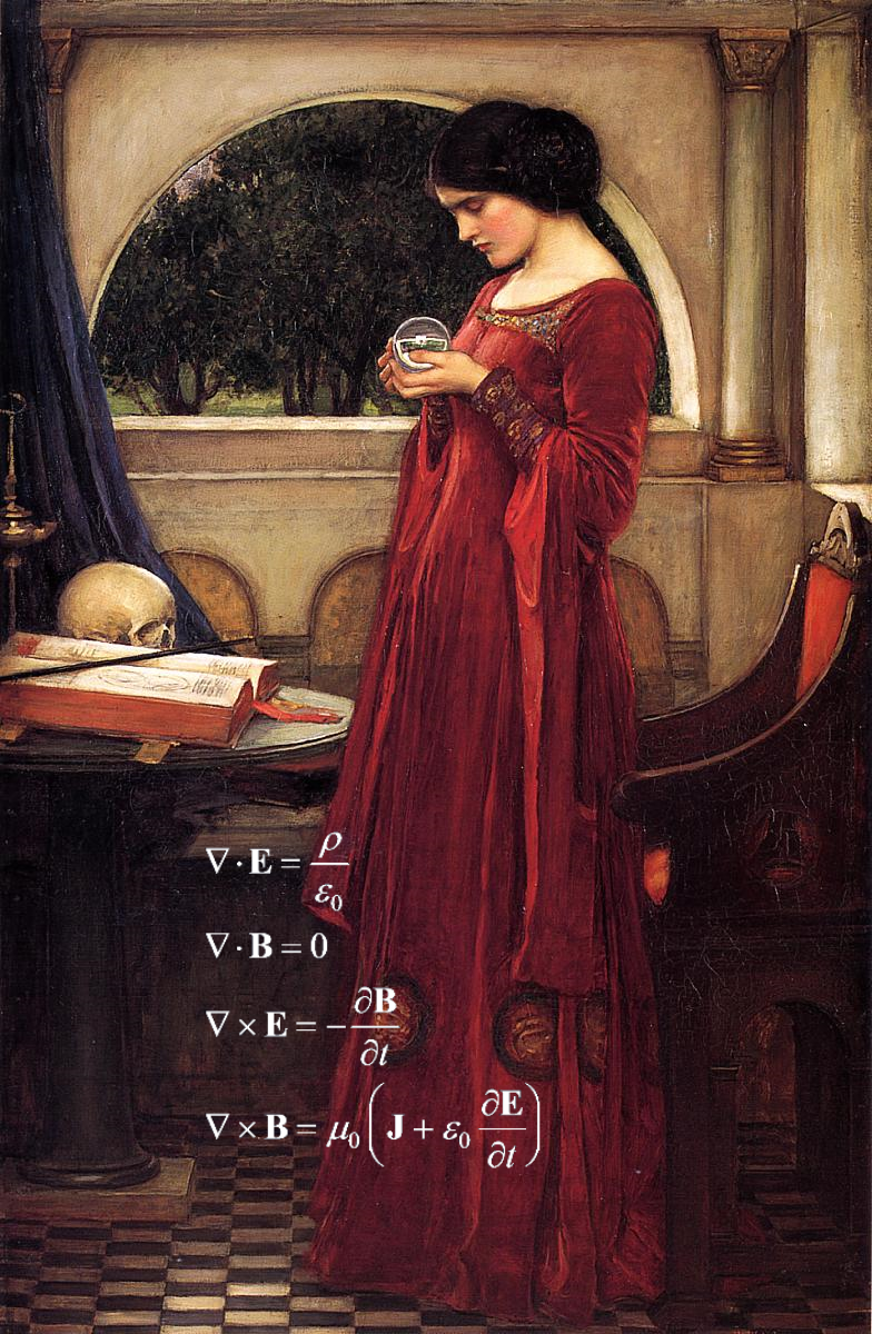
Much like a crystal ball, Maxwell's equations can predict the behavior of electromagnetic phenomena. Background image by John William Waterhouse and in the public domain via Wikimedia Commons.
Much like a crystal ball, Maxwell's equations can predict the behavior of electromagnetic phenomena. Background image by John William Waterhouse and in the public domain via Wikimedia Commons.
Expressing the Laws of Physics with Mathematics
When we look at how the laws of physics are expressed in terms of PDEs, there are some mathematical concepts that we need to be familiar with in order to understand the meaning of the equations. In many cases, conservation laws can be expressed using the divergence of a vector field (or tensor); for example, in a flux where the vector is given by a constitutive relation.
The divergence of a vector, J, is expressed as follows:
(1)

We can see from this equation that the divergence takes the sum of the changes of the vector field in the different directions. If the flux of a physics quantity is conserved, then the sum of the changes in all directions is zero, so that F is zero in the equation below:
(2)

This equation was derived in an intuitive way by Gauss. He took the sum of the fluxes over a surface that encloses a volume and balanced this with the volumetric sum of the sources or sinks (F). Letting the volume approach zero yields the differential equation. This derivation is referred to as Gauss’s theorem or the divergence theorem.
Let us assume that the vector J represents electric current density. If the divergence of the current density vector is zero, then the change of the current density in one direction is perfectly balanced by changes in the other directions at every point in the modeled domain, so that electric charge is conserved at every point.
The curl of a vector describes the rotation of a three-dimensional vector field. It can be derived as the circulation area density of a vector field at every point in a domain:
(3)

For example, the vorticity of a fluid at every point in a domain is given by the curl of the velocity vector. If we look at a very small control volume in the fluid domain with a flow of nonzero vorticity, the curl gives the direction of the rotation axis and the magnitude of the rotation for the control volume. For irrotational flows, the curl of the velocity field is zero.
The curl of flux vectors is also used in Maxwell’s equations. For example, it is used to describe Faraday's law of induction, where the curl of the electric field, due to a temporal change in the magnetic flux density, can be expressed as follows:
(4)

The gradient operator is the last mathematical concept in this section. It is often used to express constitutive relations; for example, for Fourier’s law for heat conduction, Ohm’s law for the conduction of electric current, and Fick’s laws of diffusion.
The gradient is a vector whose components give the slope of, for example, a scalar field in different directions:
(5)

The slope can, in its turn, give the flux in the constitutive relations mentioned above. For example, Fourier’s law for heat conduction gives a heat flux with direction and magnitude that is proportional to the gradient of the temperature, with the thermal conductivity as the proportionality constant:
(6)

The analogies for Ohm’s law and Fick’s first law of diffusion give the electric current density as the negative of the gradient of the electric potential for static electromagnetic fields, Φ, with the electric conductivity as the proportionality factor; the flux of chemical species as the negative gradient of the concentration, c; and the diffusion coefficient as the proportionality factor, respectively:
(7)

If we look at the equations used in engineering and science for describing physical systems, the laws are expressed as PDEs. Mathematical models may be defined using a combination of the definition of the laws and a bunch of constitutive relations that describe the phenomena involved in the described physical system.
The World as We Observe It
In the paragraphs below, we discuss a few of the laws used in engineering and science. The equations included in these laws also form the basis of multiphysics modeling and simulation, and they are hence related to the way in which we observe physical phenomena. As mentioned above, constitutive relations introduce concepts such as diffusivity, conductivity, and density. These quantities are defined via the continuum assumption, which states that there exists a volume such that a measurement with this sensitive volume gives a "local" representation of the measured property, and a small reduction in volume size must not change the average. The continuum hypothesis is illustrated in the graph below.
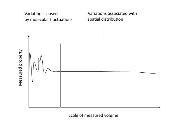 The value of a measured property depends on the sensitive volume of the measurement.
The value of a measured property depends on the sensitive volume of the measurement.
The value of a measured property depends on the sensitive volume of the measurement.
The continuum hypothesis is valid for most engineering applications and it allows us to describe fluids and solids as being continuous media rather than collections of individual atoms. For very small equipment or apparatuses, however, there might not exist any volume small enough to be considered a point, compared to the size of the equipment, and large enough to average out molecular variations. This implies that the variations caused by molecular fluctuations to the left in the figure above and the large scale variations to the right overlap. The effects that can be observed under such circumstances are referred to as rarefication effects. Most of the laws described below do not account for these effects. On even shorter length scales, we may encounter quantum effects. Some applications that we use in everyday life make direct use of quantum effects; for example, semiconductors. Quantum effects are briefly discussed below. Another type of effect that may be observed in engineering applications is relativistic effects, which are briefly mentioned below. Note, though, that even with relativistic effects taken into account, the laws of physics can be expressed in terms of PDEs.
The Schrödinger Equation
The Schrödinger equation is based on the law of conservation of energy of a system, with the probability density being the conserved quantity. In quantum mechanics, the solutions to the Schrödinger equation, the wave functions, result in probability functions for the position of elementary particles in time and space through linear combinations of wave functions. In most cases, the wave functions exist for quantized energy levels; that is, only specific discrete values may occur. For example, electron density wave functions result in orbital probability functions for atoms and molecules.
Let us look at an example of the formulation of the Schrödinger equation for the hydrogen atom:
(8)

In this equation, ψ denotes the wave function, ħ the reduced Planck constant, Ĥ the Hamiltonian operator, and i the unit imaginary number.
The Hamiltonian reads as follows:
(9)

Here, me denotes the electron's mass and V(r) the potential energy as a function of a radial vector r.
For definite energy states, we can rewrite the equation wave function according to the following:
(10)

which, in time-harmonic form, gives:
(11)

The potential energy, V, for the electron depends only on the radius, and the wave function can be formulated in spherical polar coordinates:
(12)

The eigenfunctions of the time-independent Schrödinger equation — that is, the wave functions with definite energy values — can be expressed as products of radial functions Rnl(r) and the spherical harmonics, Ylm. Here, n is known as the principal quantum number, l denotes the quantum number for the orbital angular momentum, and m refers to its z-component. It is found that the energy levels depend only on n; that is, E(ψnlm) = En. The following figure shows some examples of the wave functions obtained by solving the Schrödinger equation in cylindrical coordinates.
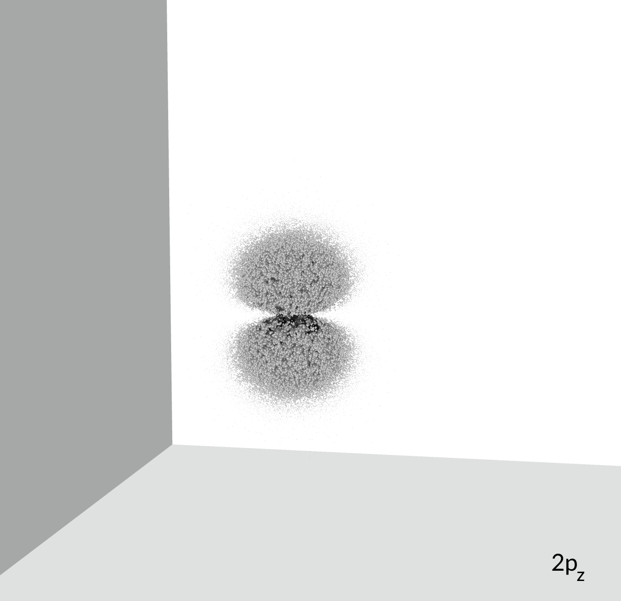
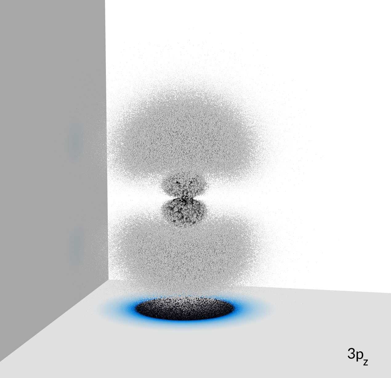
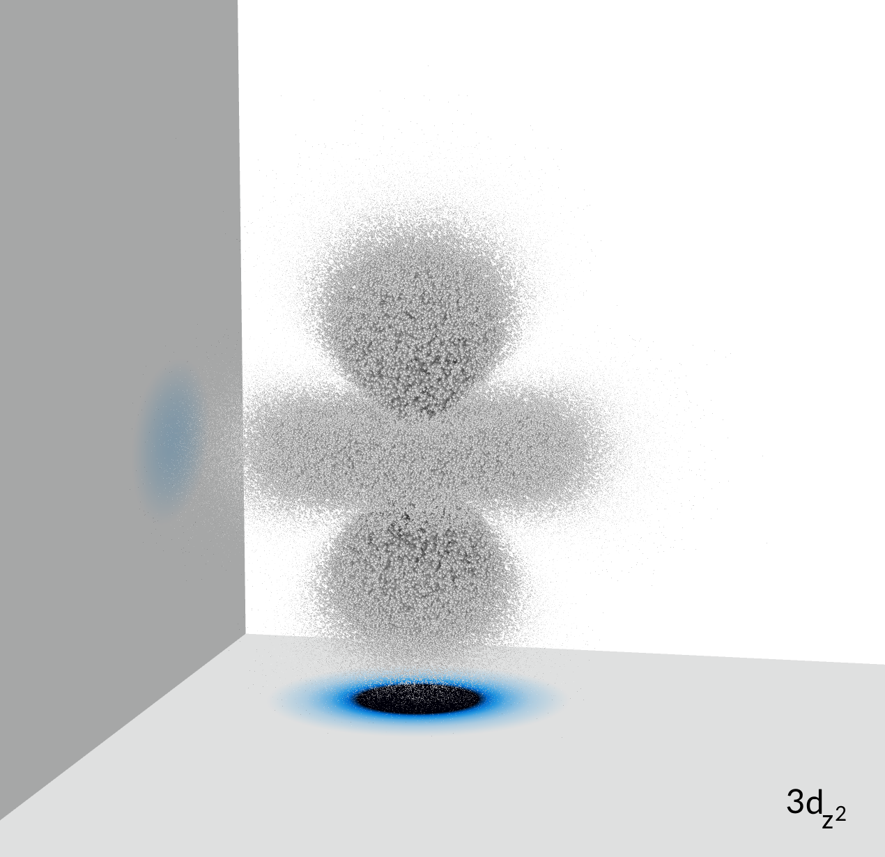
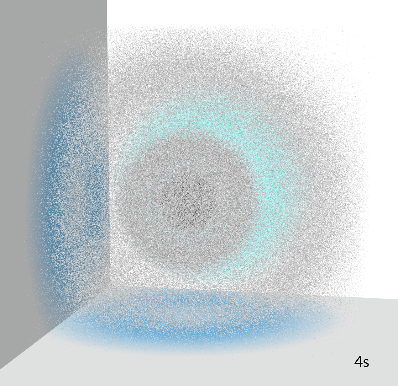


Wave functions (probability functions for the position) with definite values of the quantum numbers n, l, and m for single electrons are called orbitals. Linear combinations (superpositions) of wave functions are also solutions to the Schrödinger equation for the hydrogen atom. The orbitals with the quantum number l = 0, referred to as s orbitals, are always spherically symmetric. Orbitals with l = 1 are denoted p orbitals and show a clear angular dependency. Orbitals with l = 2 are called d orbitals, which show an even more complicated angular dependency. The plots show the probability density visualized by particles, where higher density and darker color indicates a higher probability density.
Using the Schrödinger equation, physicists and physical chemists have been able to compute the table of elements with the possible stable elements in this universe.
The measurement of a particle’s position and time is associated with an uncertainty that says that the more precisely the particle’s position is determined, the less precisely its momentum can be determined. This is known as the Heisenberg uncertainty principle after the scientist who formulated it. For example, if the position of a particle is known exactly, its momentum cannot be determined at the same time.
In quantum mechanics, wave function collapse occurs when the position or momentum is observed. This can also be explained by decoherence when a particle interacts with its environment. This means that when a particle is measured, the wave function no longer describes it (or appears to no longer describe it, according to decoherence) and the particle will be found in only one place. Schrödinger's cat is a famous abstraction of this concept. When the box is closed, the cat is both dead and alive. When we open the box, the cat is either dead or alive.
Schrödinger's equation has a large number of applications for chemistry and physics. It is also used in the semiconductor and electronic industries to account for quantum effects in devices and processes. The Schrödinger–Poisson equations are widely used for the description of quantum dot displays and semiconductor devices based on quantum dots. These equations combine the Schrödinger equation with a balance of charge (see Gauss's law in the Maxwell equations section below), where the electric potential from the balance of charge contributes to the potential energy term in the Schrödinger equation.
Before leaving the topic of the Schrödinger equation, let us make a brief digression on quantum theory and special relativity. With suitable reinterpretations of the wave function ψ and the Hamiltonian Ĥ, Paul Dirac was able to formulate a wave equation — now named after him — that is compatible with the special theory of relativity. Applied to the hydrogen atom, ψ in the Dirac equation is a so-called bispinor with four complex-valued components. It has solutions that correspond to electrons associated with an intrinsic angular momentum, the spin, with values +ħ/2 ("spin up") and -ħ/2 ("spin down"), respectively. Now, the energy levels no longer directly depend only on the principal quantum number n, but rather on n and the total angular momentum quantum number, j, where the quantum numbers j, l, and s (the spin quantum number) satisfy the constraints |l – s| ≤ j ≤ l + s. The splitting of the hydrogen atom's energy levels for orbitals with the same value of l but different values of j (and hence s) is known as fine structure. Historically, it had been observed in the spectral lines of hydrogen before the Dirac equation provided a theoretical basis. However, it was clear early on that the Dirac equation was not the last word in the mathematical formulation of quantum physics. The existence of negative-energy solutions led to the prediction of antiparticles (the positron), and problems with the interpretation of the vacuum state followed. Eventually, these issues were resolved by the development of quantum field theory, which forms the basis of modern elementary particle physics and has further applications in condensed matter physics, to mention just two important contemporary fields of study.
Maxwell's Equations of Electromagnetism
Maxwell’s equations describe the laws of electricity and magnetism that, when combined, also describe light and any other type of electromagnetic radiation. Feynman once made a funny remark in one of his lectures in reference to the Book of Genesis in the Bible. He said that Maxwell, when discovering these equations, could have said: “Let there be electricity and magnetism, and there is light!” In a way, his statement describes the importance of Maxwell’s discovery for science and engineering.
The first of Maxwell’s equations that we will look at is Gauss’s law:
(13)

Gauss’s law describes a balance of charge. It states that the electric flux density is balanced by the net charge in every point in a modeled domain. It can be derived from Gauss’s theorem, where the integral of a flux of a quantity across a closed surface equals the net source of that quantity in the volume enclosed by the surface. Letting the volume approach zero gives the differential equation from the integral equations. This theorem is also referred to as the divergence theorem, which is introduced above in Eq. (2).
The second equation, below, is usually referred to as Gauss’s law for magnetism:
(14)

This equation simply states that magnetic flux is conserved at every point in the modeled domain. (Eq. (2)) In other words, magnetism is a source-free field.
The third equation here is the so-called Maxwell–Faraday equation. The differential equation can be derived from the more intuitive integral equation, which is a mathematical description of Faraday’s law of induction:
(15)
This equation states that if we take the sum of the electric field over the path of a closed loop in a domain, then this net sum must be perfectly balanced by a temporal change in the magnetic flux across the surface enclosed by that loop. The inverse interpretation is, of course, equally viable and may be easier to recognize: A time-varying magnetic flux density will cause a net voltage in a loop around the plane perpendicular to the magnetic flux density.
In this instance, we are talking about induction. For example, a time-varying magnetic flux caused by a moving magnet will cause a current in the copper winding around the magnet; i.e., a current is induced in the coil. Faraday observed this phenomenon experimentally and Maxwell later described it in his equations.
The last of Maxwell's equations describes Ampère’s circuital law:
(16)

This equation says that a current and a time-varying electric field cause a circulating magnetic flux around a plane perpendicular to the current and electric field. For example, a current in a copper wire causes a circulating magnetic flux in the wire.
Maxwell’s equations with moving frames are compatible with special relativity. However, for accelerating charges, the use of these equations requires some care. The origin of the reaction force for accelerating charges is still an area of research and implies marrying gravity with quantum electrodynamics.
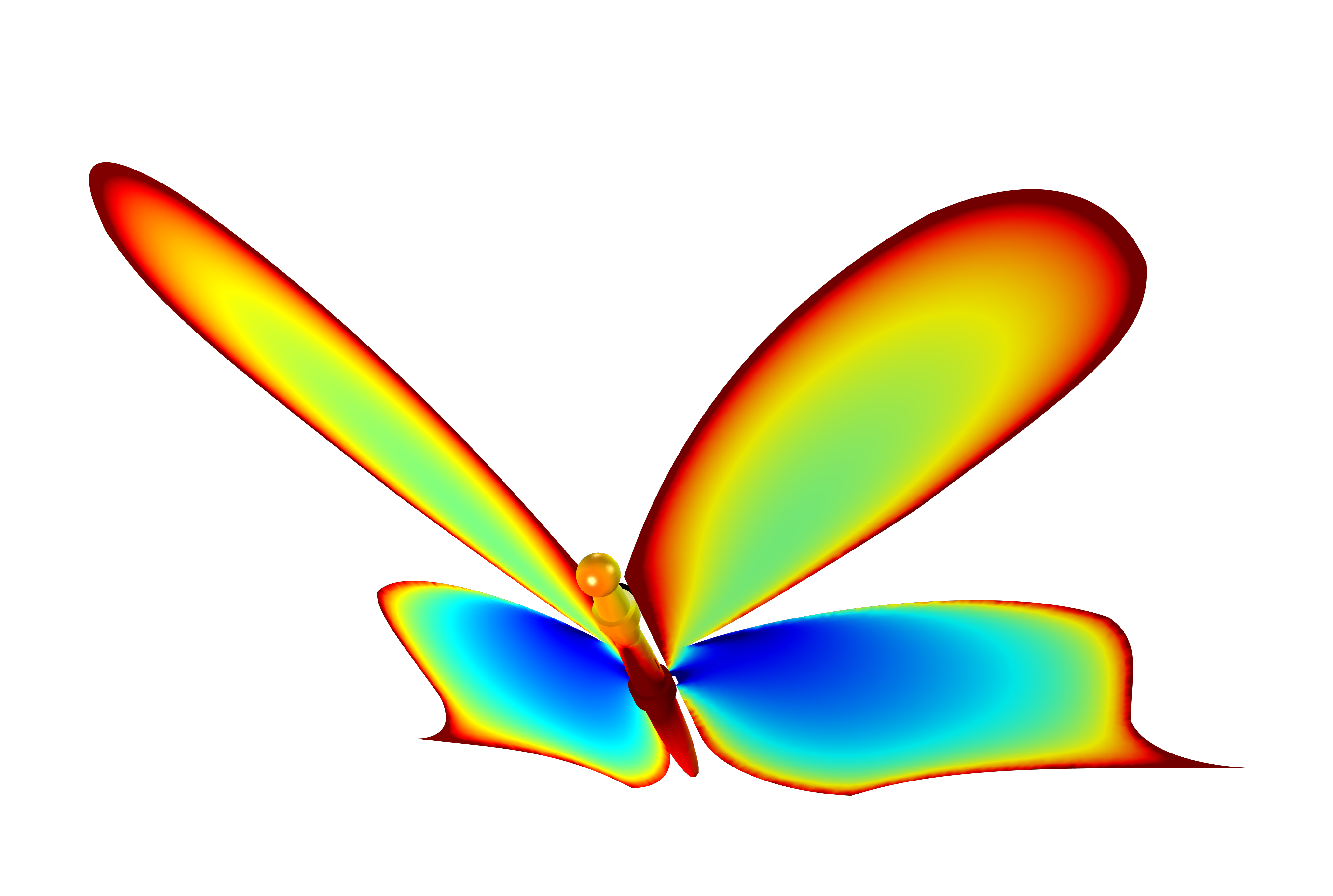 A simulation of a robotic butterfly, where the dielectric body and conductive wings work as an efficient RFID system. Maxwell's equations form the basis of this type of simulation.
A simulation of a robotic butterfly, where the dielectric body and conductive wings work as an efficient RFID system. Maxwell's equations form the basis of this type of simulation.
A simulation of a robotic butterfly, where the dielectric body and conductive wings work as an efficient RFID system. Maxwell's equations form the basis of this type of simulation.
This is just a scratch on the surface of the implications of Maxwell’s equations. There are many other equations and models that can be defined through different assumptions and simplifications about electromagnetic fields. (Ref. 2) For example, AC fields usually follow a sinusoidal temporal variation. For these cases, we perform a Fourier transform, which transforms the equations from the time domain to the frequency domain. We then obtain a set of stationary equations in terms of complex-valued functions to describe the electromagnetic fields instead of time-varying, real-valued functions.
You can find a complete introduction to the theory behind electromagnetics here.
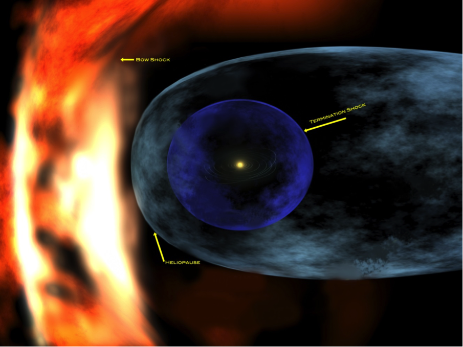
The solar wind, consisting of charged particles and the magnetic field from the Sun, protects the solar system from cosmic rays (charged particles from deep space). This effect is partly explained by Maxwell’s equations. Image in the public domain via NASA.
The solar wind, consisting of charged particles and the magnetic field from the Sun, protects the solar system from cosmic rays (charged particles from deep space). This effect is partly explained by Maxwell’s equations. Image in the public domain via NASA.
The Equations of Motion for Solid Mechanics
Newton's second law explains that a force is required to change the velocity of a body. For example, this law can be used to express a force balance. For the forces inside a solid body, this balance of forces yields a local acceleration that is counteracted by internal stresses or by any volumetric force. Ref. 3 The equations of motion for solid materials, according to Newton's second law, are the following:
(17)

where σ denotes the stress tensor according to:
(18)

and u is the displacement vector u = (u, v, w).
We take the divergence of a tensor, which yields the following vector:

For an elastic material, we can obtain the stresses from a general formulation of Hooke's law; i.e., the constitutive relation:
(19)

where D denotes the constitutive matrix on the stiffness form and ε denotes the strains according to:
(20)

The system of partial differential equations in Eq. (17), together with the constitutive relations in Eq. (19), is valid for linear materials. When combined with the expressions for the strain components, they give Navier's equations, which can be written as:
(21)

E denotes the modulus of elasticity and ν is Poisson's ratio.
Poisson's ratio is obtained by dividing the relative expansion of a material, perpendicular to the direction of an applied compressing force, with the relative compression. The corresponding general balance of forces for a so-called nonlinear material model can be written in a similar way.
Although it sounds pretty limited, the equations for linear materials are very common. This is simply because in most cases, engineers do not want plasticity, which is when components do not go back to their original shape once a load has been removed. When designing mechanical components, the bulk of the material should work in the elastic region so that the component goes back to its original shape when it is not subjected to forces. Edge effects that may lead to plasticity are usually confined to small regions of the component.
Find a complete introduction to structural mechanics here.
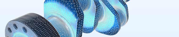
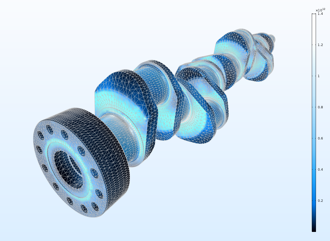 Stresses in a crankshaft for a six-cylinder engine, computed with the finite element method, which solves a numerical approximation of the PDEs discussed above.
Stresses in a crankshaft for a six-cylinder engine, computed with the finite element method, which solves a numerical approximation of the PDEs discussed above.
Stresses in a crankshaft for a six-cylinder engine, computed with the finite element method, which solves a numerical approximation of the PDEs discussed above.
The Equations for Conservation of Mass and Chemical Species Transport
The time rate of change of the mass concentration of a chemical species has to be balanced by the change in flux and the production or consumption of that species in a control volume. (Ref. 4) This is expressed in the following equation:
(22)

In this equation,  denotes mass concentration (SI unit kg/m3) of the ith species;
  denotes the mass flux vector;
  is the molar mass; and
  is the reaction rate, with respect to the ith species, for all reactions that produce or consume this species.
The flux of chemical species can be described with constitutive relations; for example, through Fick's first law of diffusion or through the Maxwell-Stefan equations. These relations or laws have their origin in a balance of forces between the driving force, created by a gradient in chemical potential, and the friction that chemical species are subjected to when they interact with each other in a solution. For a binary solution, where only two species are present, the material balance equations become:
(23)

where  denotes the diffusivity in the binary solution (
 and
and  ).
).
For a concentrated solution with more than two species, the description of diffusion becomes somewhat more complicated. For dilute solutions, the expression for diffusion is similar to the binary solution, with the interactions between each solute species and the solvent as the only relevant interactions. The drawing below shows the difference in the interactions that have to be accounted for in the case of dilute and concentrated solutions.
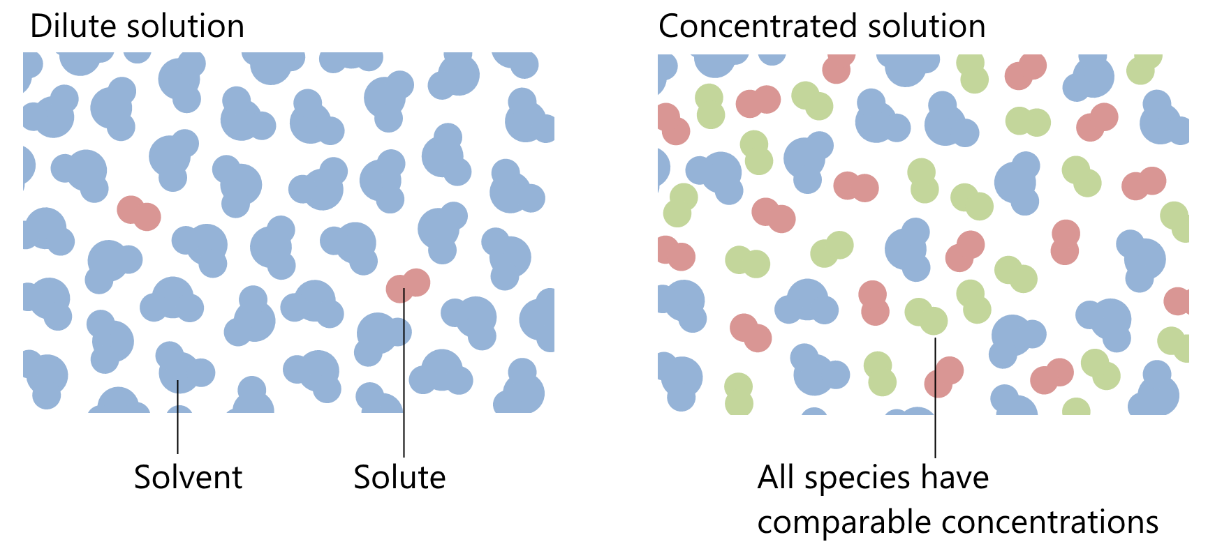 A schematic drawing that shows the implications on interactions for dilute and concentrated solutions.
A schematic drawing that shows the implications on interactions for dilute and concentrated solutions.
A schematic drawing that shows the implications on interactions for dilute and concentrated solutions.
The mass balance equations for each chemical species are usually solved in combination with the momentum equation for fluid flow, which is presented in the next section. In a concentrated solution, the sum of all material balances yields the continuity equation for conservation of mass. The reaction terms for the chemical species cancel out, since chemical reactions preserve mass:
(24)

Note that the sum of all diffusive mass fluxes over all species is also zero, since diffusion represents the deviation of the mass flux of a species in relation to the mass-averaged velocity of an advected control volume; i.e., when we "follow along" with the flow. For a concentrated solution, the mass-averaged velocity is defined as:
(25)

For a dilute solution, the velocity is given by the velocity of the solvent.
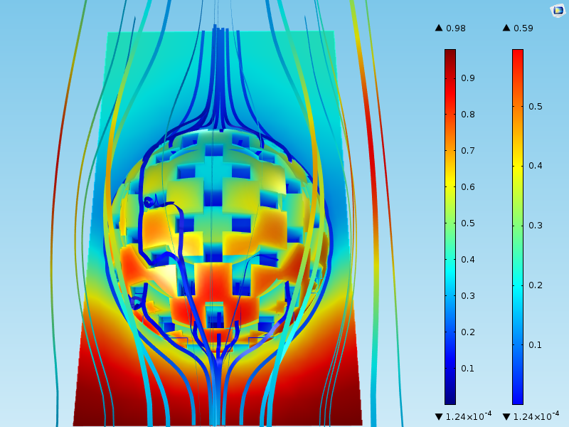 A dimensionless concentration of a reacting species (1 at the inlet) in and around a catalyst particle modeled using the mass balance equations and the equations for fluid flow.
A dimensionless concentration of a reacting species (1 at the inlet) in and around a catalyst particle modeled using the mass balance equations and the equations for fluid flow.
A dimensionless concentration of a reacting species (1 at the inlet) in and around a catalyst particle modeled using the mass balance equations and the equations for fluid flow.
The mass balance equations are often solved in combination with the equation for conservation of momentum, as explained below. These sets of equations are used to understand, predict, and optimize the design and operation of biochemical devices, chemical reactors, batteries, fuel cells, environmental processes and systems, and combustion, to mention a few examples.

Processes in chemical plants are often designed with the help of modeling using the mass balance equations. Image by Maarten Takens. Licensed under CC BY-SA 2.0, via Flickr Creative Commons.
Processes in chemical plants are often designed with the help of modeling using the mass balance equations. Image by Maarten Takens. Licensed under CC BY-SA 2.0, via Flickr Creative Commons.
The Equations of Motion for Fluid Mechanics
The equations for conservation of mass and momentum form the basis for the modeling of fluid flow. (Ref. 4) Fluid flow modeling, for example, in computational fluid dynamics (CFD), is involved in the understanding of designs and processes from spaceships to chemical plants.
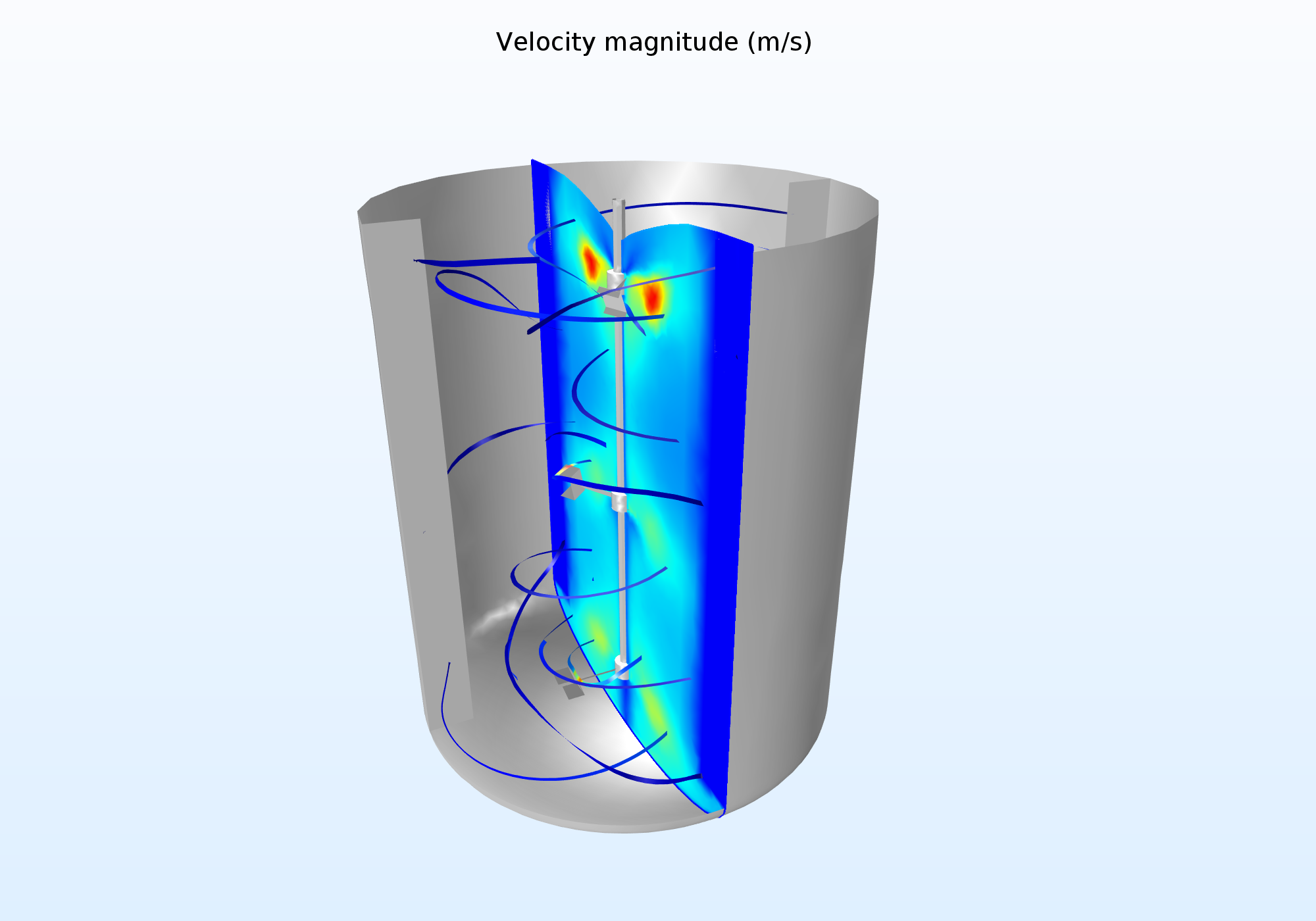 Simulation results of the fluid flow in a chemical reactor equipped with three central impellers and four baffles attached to the reactor walls. The baffles impede a "merry-go-round flow", thus inducing mixing in the radial direction.
Simulation results of the fluid flow in a chemical reactor equipped with three central impellers and four baffles attached to the reactor walls. The baffles impede a "merry-go-round flow", thus inducing mixing in the radial direction.
Simulation results of the fluid flow in a chemical reactor equipped with three central impellers and four baffles attached to the reactor walls. The baffles impede a "merry-go-round flow", thus inducing mixing in the radial direction.
The equations of motion for a fluid are quite similar to the equations for solids. Once again, we start from Newton's second law. Since momentum is a vector, we get the following vector equation for conservation of momentum:
(26)

In this equation,  denotes the momentum flux tensor,
  is the total stress tensor and
  is a volume force; for example, due to gravity.
The first term on the left-hand side of the equation above represents the rate of change of momentum per unit volume, and the second term results from the advective transport of momentum. The first term on the right-hand side results from forces acting on each side of a surface element in the fluid, and the last term is the sum of forces acting per unit volume of the fluid.
The momentum flux tensor is given by:
(27)

The total stress tensor is usually divided up into the pressure and a deviatoric part, which basically contains everything else:
(28)

where  is a tensor with ones on the diagonal and zeros everywhere else.
In general, the deviatoric stress is a full tensor:
(29)

For a Newtonian fluid, the deviatoric stress, also called the viscous stress, is symmetric (so that for, example the  and
and  components are equal) and proportional to the rate of strain:
(30)

In the above equations,  denotes shear viscosity and
  is the dilatational, or bulk, viscosity (often ignored).
The equation for conservation of momentum becomes:
(31)

With the aforementioned linear relation between the viscous stress and the strain rate, this equation is commonly known as the Navier–Stokes equation. The Navier–Stokes equation introduces three dependent variables for the velocity components ( ), one for the pressure (
 ), and one for the density (
 ), while only providing three equation components.
The three components of the momentum equation are usually solved in combination with the equation for conservation of mass (the continuity equation):
(32)

For a fluid of constant composition and temperature, the equations for conservation of momentum and mass may be supplemented with an equation of state to obtain a closed system of equations. The equation of state constitutes the additional relation between pressure and density. For gases, we can use the ideal gas law, which expresses density as a function of pressure at a given temperature. This gives five unknowns ( , and ) and five equations (the three components of the momentum equation, the continuity equation, and the equation of state).
For flows with appreciable variations in composition or temperature, additional equations for species transport or heat transfer must be solved together with these five equations.

The equations for fully compressible flow are usually required to model the fluid flow around fighter jets, like this F/A-18 Hornet. The shockwave, formed as the aircraft breaks the sound barrier, gives rise to condensation that forms a small cloud around the jet. U.S. Navy photo by Ensign John Gay; in the public domain via Wikimedia Commons.
The equations for fully compressible flow are usually required to model the fluid flow around fighter jets, like this F/A-18 Hornet. The shockwave, formed as the aircraft breaks the sound barrier, gives rise to condensation that forms a small cloud around the jet. U.S. Navy photo by Ensign John Gay; in the public domain via Wikimedia Commons.
For constant density and viscosity, the Navier–Stokes and continuity equations can be further simplified to yield the following four-equation system for the velocity and pressure:
(33)

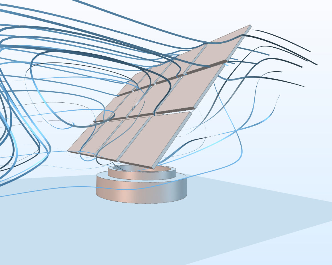 The airflow around a solar panel is modeled using the incompressible form of the Navier–Stokes and continuity equations. The forces exerted by the wind on the surface of the panels can be used as loads in a structural analysis of the panel.
The airflow around a solar panel is modeled using the incompressible form of the Navier–Stokes and continuity equations. The forces exerted by the wind on the surface of the panels can be used as loads in a structural analysis of the panel.
The airflow around a solar panel is modeled using the incompressible form of the Navier–Stokes and continuity equations. The forces exerted by the wind on the surface of the panels can be used as loads in a structural analysis of the panel.
Solutions of this so-called incompressible form of the Navier–Stokes and continuity equations describe flow fields with a wide range of complexity, from reversible creeping flow to chaotic turbulent flow, which, by Feynman's account, is "the most important unsolved problem of classical physics."
If we further neglect the time rate of change and advection of momentum, we obtain the so-called Stokes equation for creeping flows.
If we instead simplify the Navier–Stokes equations by neglecting the viscous forces (inviscid fluid model), we obtain the Euler equations:
(34)

In a later, more general definition of the Euler equations, the momentum balance for fully compressible flow (not constant density) in Eq. (31) is coupled with the mass conservation equation, Eq. (32), and the equation for conservation of energy, Eq. (38). However, the conductive term and the viscous dissipation are usually neglected.
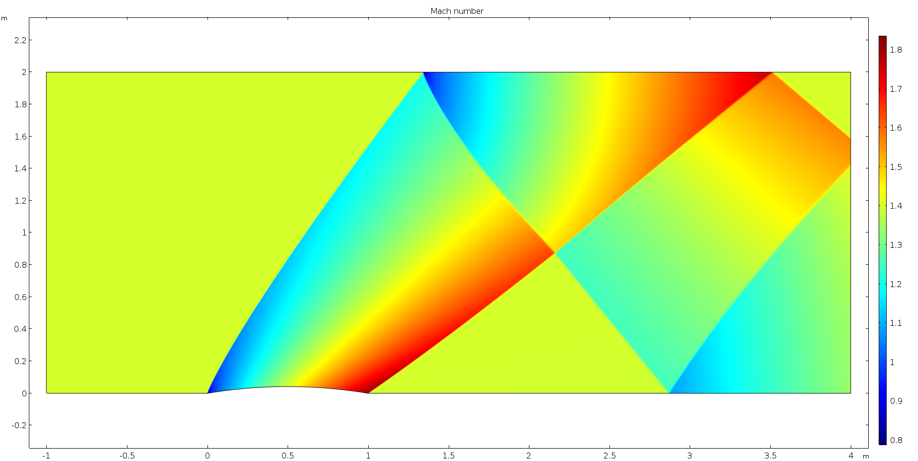
A diffraction pattern in a Mach number plot arising from supersonic flow hitting a small, wing-profile-shaped obstacle in its path. (Ref. 5)
A diffraction pattern in a Mach number plot arising from supersonic flow hitting a small, wing-profile-shaped obstacle in its path. (Ref. 5)
For confined gases at low pressures, the mean free path of the gas molecules can be much larger than the size of the modeled system. In such cases, the continuum hypothesis mentioned above is no longer valid. Models for such systems are based on kinetic theory of gases. The theory for free molecular flow is based on a velocity distribution of the gas molecules colliding with each other and with the walls of the system, where the velocity is described by a Maxwell–Boltzmann distribution. At very low gas pressures, the gas molecules only collide with the walls of the system. At a certain gas molecule concentration (pressure) in a system, collisions between particles have to be taken into account. If these collisions are about as common as the collisions with the walls of a system, the velocity function has to include these collisions. The Boltzmann equations or the Boltzmann BGK equations (a simplified form of the Boltzmann equations) can be used to model flow in this transitional region. When the mean free path is one tenth or less than the size of the system, then the rarefication effects only need to be accounted for a very thin layer close to the walls: the so-called Knudsen layer. These models are referred to as slip flow models. In the continuum flow regime, the Navier–Stokes equations are applicable. The effect of the Knudsen layer can be modeled using special boundary conditions for the Navier–Stokes equations.
The ratio of the molecular mean free path to the size of the system (l) is given by the Knudsen number (Kn = λ/l). There are four flow regimes depending on the value of the Knudsen number:
- Continuum flow: Kn ≪ 0.01
- Slip flow: 0.01 < Kn < 0.1
- Transitional flow: 0.1 < Kn < 10
- Free molecular flow: Kn > 10
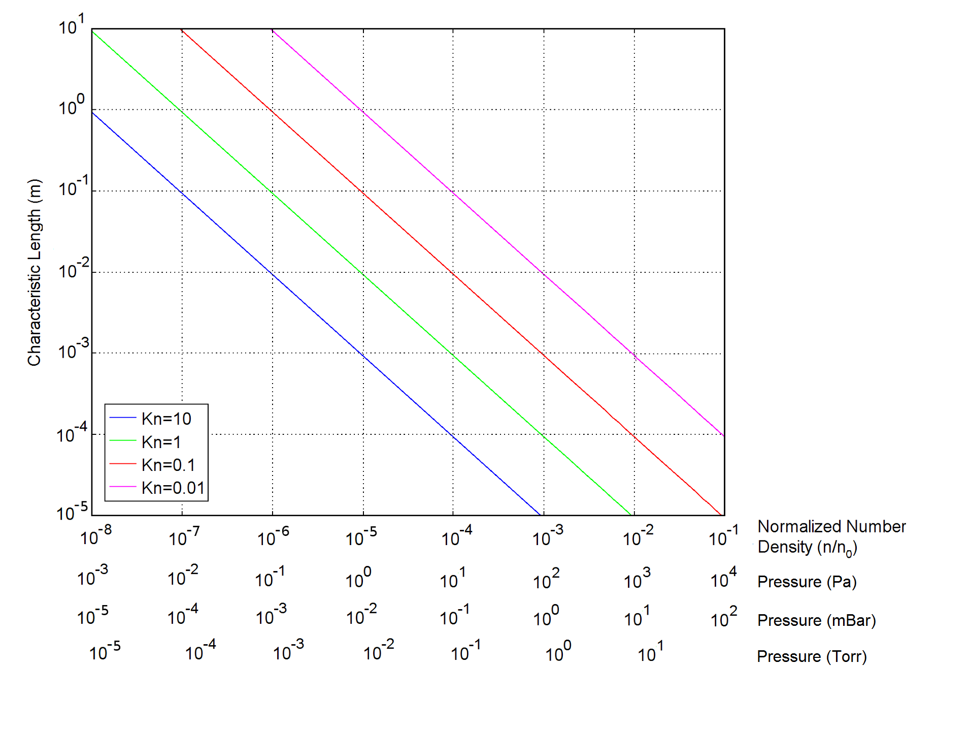 The flow regimes as determined by the Knudsen number.
The flow regimes as determined by the Knudsen number.
The flow regimes as determined by the Knudsen number.
The Heat Transfer Equation and the Energy Equation
The first law of thermodynamics defines the internal energy by stating that the change in internal energy for a closed system, ΔU, is equal to the heat supplied to the system, Q, minus the work done by the system, W:
(35)

If the system is allowed to move, Eq. (35) can be extended to include the kinetic energy for the system,  :
:
(36)

 The equation for the change of temperature can be used to predict the temperature distribution in heat sinks. Such analyses can be used for electronic cooling purposes, to design heat sinks, and to determine how cooling should be applied in a process.
The equation for the change of temperature can be used to predict the temperature distribution in heat sinks. Such analyses can be used for electronic cooling purposes, to design heat sinks, and to determine how cooling should be applied in a process.
The equation for the change of temperature can be used to predict the temperature distribution in heat sinks. Such analyses can be used for electronic cooling purposes, to design heat sinks, and to determine how cooling should be applied in a process.
(37)

The result is known as the equation for conservation of total internal energy, (Ref. 4). In this equation:
- ρ is the density
- e is the internal energy per unit mass
- v is the velocity vector
- v2 is the square of the velocity magnitude
- q is the conductive heat flux vector
- σ is the total stress tensor
- F is the body force per unit mass, i.e., the volume force
Still, for a fluid, we can invoke the momentum equations Eq. (31) and the continuity equation Eq. (24) and reduce Eq. (37) to an equation for the conservation of internal energy:
(38)

where is the pressure and  is the viscous stress tensor (see Eq. (30)).
A more convenient way to express conservation of energy is to rewrite equation Eq. (38) in terms of temperature. Temperature can be measured, and engineers are more used to working with temperature than with internal energy. This can be achieved by using the following thermodynamic relations:
(39)

Some algebraic manipulation, again using the continuity equation and inserting Fourier's law according to Eq. (6), yields:
(40)

The last term on the right-hand side,  , has been added to account for internal heat sources caused by reactions or interaction with radiation, for example.
Eq. (40) describes conservation of energy in a fluid. The corresponding equation for energy conservation in a solid can be derived from the first law of thermodynamics (Eq. (35)). The result reads
(41)

where  is the thermal expansion coefficient tensor;
  is the time derivative of the stress tensor;
  is the strain rate tensor; and represents all possible inelastic stresses (for example, a viscous stress).
The term  is called thermoelastic damping and corresponds to the pressure work,
  , in Eq. (40). The term
  represents viscous heating and is the solid representation of the term
  in Eq. (40). The close resemblance between the energy conservation equations is, of course, a direct effect of the fact that they both describe the same underlying conservation principles.
The heat transfer equation has applications in all fields of physics and engineering. Sometimes, heat is a desired product of a process, but in many cases, it is a byproduct of a process that has to be dissipated through cooling. In the image below, the expansion of gases created by heat of reaction (combustion) propels the space shuttle out to space. In the figure above, showing a heat sink for electronics cooling, heat has to be removed from the electronic circuit in order for it to perform properly.

The heat of reaction: The Discovery space shuttle launched from NASA’s Kennedy Space Center in 1997. Image in the public domain via Wikimedia Commons.
The heat of reaction: The Discovery space shuttle launched from NASA’s Kennedy Space Center in 1997. Image in the public domain via Wikimedia Commons.
Last modified: March 21, 2019
References
- R. Feynman, "Differential Calculus of Vector Fields", The Feynman Lectures on Physics, Caltech's Division of Physics, Mathematics and Astronomy, 2013.
- C.A. Balanis, Advanced Engineering Electromagnetics, John Wiley & Sons Inc., 1989.
- J.A. Stratton, Electromagnetic Theory, McGraw Hill Company Inc., 1941.
- Y.C. Fung, Foundations of Solid Mechanics, Prentice-Hall Inc., 1965.
- R.D. Bird, W.E. Stewart, E.N. Lightfoot,Transport Phenomena, 2nd ed., NY: John Wiley & Sons Inc., 2002.