
Introduction to Acoustics
What Is Acoustics?
Acoustics is the physics of sound, including all of the multiphysics disciplines concerned with the production, transmission, and detection of the sound signal. Sound here means not only what is detected by the human ear but also infrasound and ultrasound; that is, wave propagation with frequencies below and above the human auditory range. The definition of sound also includes the propagation in media other than air. This could be elastic waves in solids (vibrations); pressure waves in liquids, like underwater acoustics; or the combined propagation in porous materials (poroelastic waves).
For humans, sound is best understood as the sensation, as detected by the ear, of very small rapid changes in the acoustic pressure p above and below a static value. This static value is the atmospheric pressure (about 100,000 pascals at sea level). This is hearing. The amplitude of the small pressure variations that can be detected by the human ear vary from roughly 20·10-6 Pa at the hearing threshold to 600 Pa for jet engine noise. The amplitude at normal speech levels is about 0.02 Pa. The values described here are often given on the logarithmic decibel scale, relative to the hearing threshold of 20·10-6 Pa (or 20 µPa), in units of dB SPL. The logarithmic scale follows naturally from how the human auditory system experiences loudness. The sound pressure level  is defined as
(1)

where  is the root mean square (RMS) acoustic pressure measured and
  = 20 µPa is the reference pressure (also an RMS value) commonly used in air. In underwater acoustics 1 µPa is typically used as reference.
Examples of the typical (broadband) sound pressure levels associated with different situations are given in the figure below. When specifying a level, it is important to specify the reference pressure, distance from the source, bandwidth measured, and possible weighting functions. As a rule of thumb, the level decreases by 6 dB each time the distance from a source is doubled. This is known as the inverse distance law.
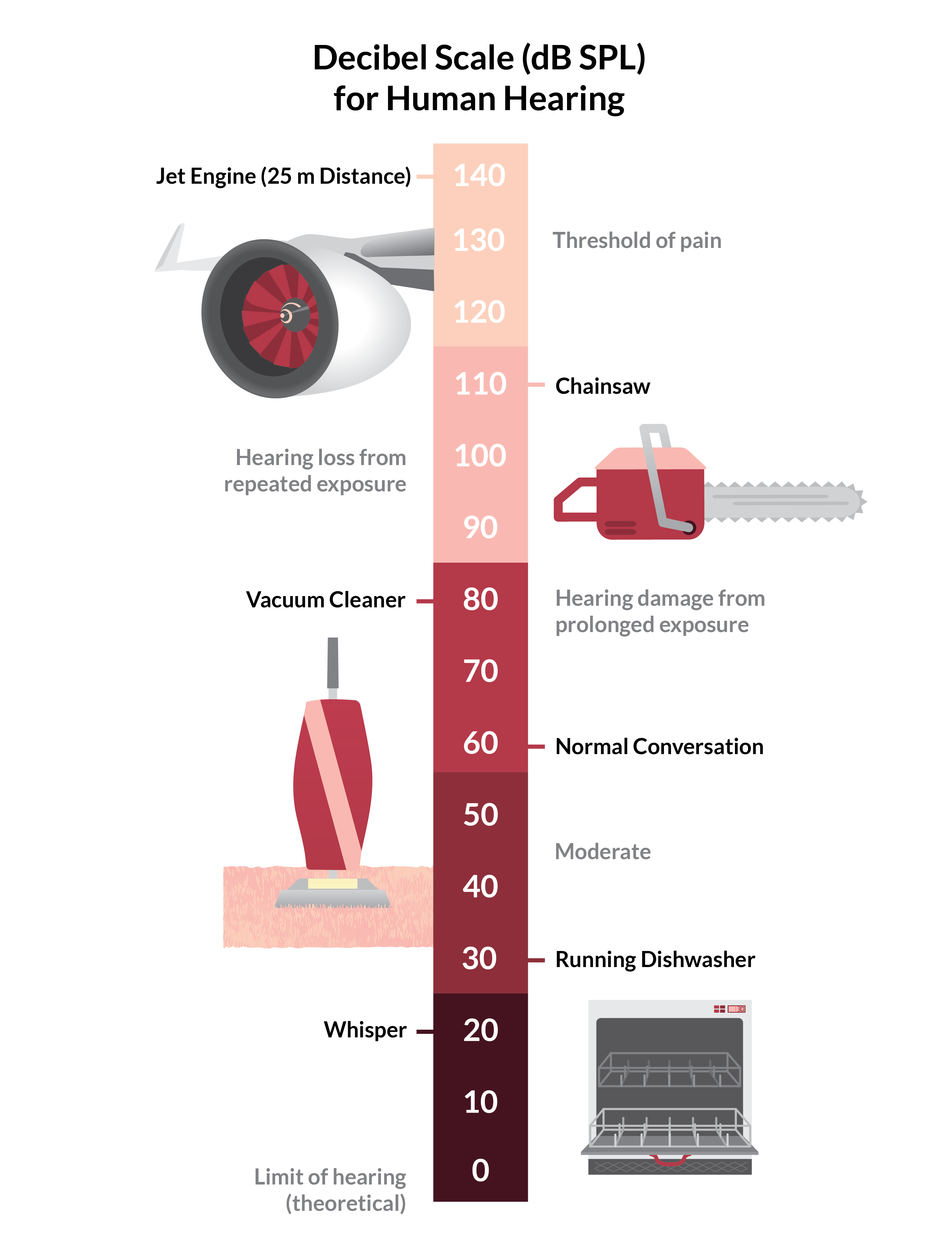
A decibel scale that illustrates the sound pressure level associated with different situations. These are typical broadband values measured in the vicinity of the source (if not stated differently).
A decibel scale that illustrates the sound pressure level associated with different situations. These are typical broadband values measured in the vicinity of the source (if not stated differently).
The waves can be propagating, standing, or a combination of both. The figure below illustrates a standing wave and a propagating wave. Wave crests are the pressure maxima, while the troughs represent the pressure minima.

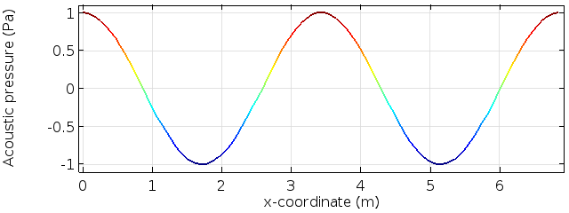
Representation of a standing wave (top) and a propagating wave (bottom).
The speed at which the waves propagate is the speed of sound  (SI unit: m/s). Its value is related to the compressibility
  (SI unit: m2/N or 1/Pa) and the density
  (SI unit: kg/m3) of the material in which the waves propagate, by
  . The speed of sound in air is about 343 m/s and 1485 m/s in water. The precise value depends on ambient temperature and pressure, as well as other variables.
To better understand the nature of standing and propagating waves, it can be very illustrative to visualize the motion of the air molecules associated with the wave. The figure below once again illustrates a standing wave (top) and a propagating wave (bottom). The background color represents the pressure amplitude (red is high and blue is low). The points represent the motion of the air associated with the waves. (Tip: Focus on one of the larger points to better understand its motion.)
Notice that even for the propagating wave, there is no net movement of an air molecule toward the right. The forward motion is that of the fluctuation that transports the energy associated with the wave. The energy transported by a wave through a cross section per unit time is the intensity  (SI unit: W/m2) of the wave.
Representation of the pressure (red is high and blue is low) and movement of air molecules for a standing wave (top) and a propagating wave (bottom).
In more general terms, sound is created when the fluid is disturbed by a source. An example is a vibrating object, such as a speaker cone in a sound system. It is possible to see the movement of a bass speaker cone when it generates sound at a very low frequency. As the cone moves forward, it compresses the air in front of it, causing an increase in air pressure. Then it moves back past its resting position and causes a reduction in air pressure. This process continues, radiating a wave of alternating high and low pressure propagating at the speed of sound (see the animation below).
Sound waves generated by a loudspeaker driver. Red represents high pressure and blue is low pressure. The movement of the loudspeaker cone is exaggerated for the purpose of illustration.
The frequency f (SI unit: Hz = 1/s) is the number of vibrations (pressure peaks) perceived per second and the wavelength λ (SI unit: m) is the distance between two such peaks. As a reference, the human auditory system (in newborns) can perceive sound with frequencies from approximately 20 Hz to 20,000 Hz (or 20 kHz). Frequency representations in octaves or fractional octave bands are very common. This is a logarithmic transform. Physiologically, such a representation is motivated by the fact that the human ear itself filters (via the auditory filters) and perceives sound on a logarithmic frequency axis. This is also a fundamental concept used in music. In the same way, the human ear also has a logarithmic sensitivity, hence the use of a decibel scale for levels, as already mentioned.
Simple Mathematical Model
Mathematically, the propagation of a sound wave along one dimension in space and time is described by the scalar wave equation
(2)

This is a partial differential equation (PDE) where t denotes time, x the spatial coordinate, c the speed of sound, and p denotes pressure (the dependent variable).
The equation is derived from the conservation laws of continuum mechanics — conservation of mass, momentum, and energy — under several assumptions that are discussed in more detail below. The general solution to the 1D wave equation is given by
(3)

where  is an arbitrary function and the sign determines if the wave is moving in the positive or negative direction.
Actually, the most general solution is a linear combination of such functions, which is known as d'Alembert's formula when initial conditions are considered. One such solution is a propagating sine wave
(4)

where  is the wave amplitude.
For the last expression, it is often convenient to define the angular frequency  (SI unit: rad/s) of the wave, which is
  , and relate the frequency to a full 360o phase shift. The wave number
  (SI unit: rad/m) is defined as
  . The wave number is usually defined as a vector, such that it also contains information about the direction of propagation of the wave. In general, the relation between the angular frequency and the wave number is called the dispersion relation; for simple fluids, it is
  . An example of a propagating wave is depicted in the animation above. The period of the oscillation is defined by
  . The product of the frequency
  and the wavelength
  is the speed of sound.
The equivalent of the wave equation formulated in the frequency domain is the all-important Helmholtz equation. The Helmholtz equation can be derived in several ways: by expanding the pressure into its Fourier components or equivalently using separation of variables (time and space). The simplest method is to assume that pressure is a time-harmonic signal of the type
(5)

where  is the complex-valued dependent variable of the problem.
Inserting this expression into the wave equation and rearranging it yields the Helmholtz equation, with constant material parameters, for a time-harmonic signal
(6)

The Helmholtz equation very often forms the basis of the numerical or analytical analysis of acoustic problems. In order to solve the wave equation or the Helmholtz equation, they should be combined with material parameters, boundary conditions, and initial conditions that describe the physical problem at hand. For more details on fundamental acoustics, see Ref. 1–4 and the Detailed Derivation of the Governing Equations section below.
The Scope of Acoustics
In acoustics, sound is produced, transmitted, and affected by the medium in which it is propagating and finally detected, perceived, and analyzed. Describing the journey of a sound signal deals with many different branches of science, including engineering, earth sciences, life sciences, and the arts.
For example, a musician reads notes and plays the piano (music). Engineers worked on the microphone that picks up the sound and other engineers optimized the reproduction of the sound by a loudspeaker (electroacoustics). Architects and civil engineers ensured that the sound is reproduced correctly in the concert hall (room acoustics). The ear of a listener picks up the sound (physiology), the sound is processed by the auditory system, and the listener perceives it as music (psychoacoustics).
Acoustics is clearly multidisciplinary and multiphysics in its nature. Here, we are primarily concerned with the physical principles of acoustics in relation to engineering and earth sciences. For a detailed classification of acoustics, see the PACS classification, as used by the Journal of the Acoustical Society of America.
A Short History of Acoustics
The first known speculations about the wave nature of sound dates back to the ancient Greek philosophers at the time of Aristotle. They were inspired by how small waves propagate at the surface of water and how they interact with obstacles as well as the generation of sound by vibrating bodies. Marin Mersenne (1588–1648) is often referred to as the father of acoustics, in particular because he gave the first correct (published) mathematical description of a vibrating string (Harmonicorum Libri in 1636). This was two years before Galileo Galilei's (1564–1642) seminal work on mechanics. During the time of Mersenne and Galileo, other physicists were not convinced by the wave nature of sound and some thought of it as a stream of matter (see Ref. 1, 21, and 22).
The first formal mathematical description of the propagation of sound in a fluid was given by Isaac Newton (1643–1727) in his work Principia (the second book from 1687). He described sound as the propagation of pulses as neighboring fluid particles interact and push each other. Newton predicted the speed of sound in air to about 298 m/s (979 ft/s), while relying on an isothermal assumption. The value and theory were later corrected by Pierre-Simon Laplace (1749–1827) in 1816 to 348 m/s (1142 ft/s), which is what you get by correcting Newton's prediction by the factor  (where
  denotes the adiabatic index; see the Linear Waves in Fluids section).
Progress toward a complete theory for the propagation of sound was made in the eighteenth century with the development of continuum mechanics and fluid dynamics through the work of Leonhard Euler (1707–1783), Joseph-Louis Lagrange (1736–1813), and Jean le Rond d'Alembert (1717–1783). The modern theory for sound propagation is, for most, based on the work of these scientists and their contemporaries. The development continued in the nineteenth century with the work of Laplace, Claude-Louis Navier (1785–1836), Siméon Denis Poisson (1781–1840), August Kundt (1839–1894), Hermann von Helmholtz (1821–1894), and George Stokes (1819–1903). Lord Rayleigh's (1842–1919) treatise The Theory of Sound from 1877 is thought to complete this long line of work with, for example, a detailed description of scattering. The work of Rayleigh is often said to mark the change from the classical to modern era in acoustics (Ref. 21–22).
Detailed Derivation of the Governing Equations
To derive the governing equations for all wave phenomena, you need to start with the conservation equations in their most general form; that is, conservation of mass, momentum, and energy. To close the system, these equations need to be supplemented by constitutive relations as well as thermodynamic equations of state.
Many different types of waves exist depending on the medium in which they propagate and their interactions. In the following sections, we derive the governing equations for waves in fluid (liquids and gases), including details about loss models and assumptions. Then, we present the governing equations for elastic waves in solids as well as the combined propagation of elastic and pressure waves in porous materials.
Conservation Equations
The conservation equations describing the motion of fluids are the continuity equation (mass conservation), Navier-Stokes equation (momentum conservation), and general heat transfer equation (energy conservation). They are given by

where the independent variables are time  (SI unit: s) and spatial coordinate
  (SI unit: m). The dependent variables are the density (SI unit: kg/m3); velocity field
  (SI unit: m/s); and entropy
  (SI unit: J/kg/K), which is the entropy per unit mass. Moreover,
  is the temperature (SI unit: K),
  is the viscous dissipation function (W/m3),
  is the total stress tensor (SI unit: N/m2),
  is the viscous stress tensor (SI unit: N/m2),
  is the local heat flux (SI unit: W/m2),
  denotes a possible mass source term (SI unit: kg/m3),
  denotes a possible heat source (SI unit: W/m3), and
  is a possible volume force source term (SI unit: N/m3). The conserved quantities here are the density , momentum
  , and total entropy
  .
.
In principle, we will consider situations where mass is conserved and so, in general,  . The acoustic perturbation to the mass source term (see below) can, however, be used as a representation for a complex process that we do not want to describe in detail.
There are many ways to write the conservation equations and select the dependent variables; above is just one of them. See, for example, Ref. 1–10 or any textbook on fluid mechanics and continuum physics.
The terms on the left-hand side of the equation represent the conserved quantities. These terms are also sometimes (after manipulations) written in a nonconservative form as

The operator  is known as the material derivative, and is defined as

Thermodynamic Relations
Some thermodynamic relations are necessary to reformulate the energy conservation equation in terms of the temperature and pressure variables. There are various ways to derive the relation; here, we present one. First, we define the (isobaric) coefficient of thermal expansion  (SI unit: 1/K); the isothermal compressibility
  (SI unit: 1/Pa); and the specific heat capacity (heat capacity per unit mass) at constant volume
  (SI unit: J/kg/K) and constant pressure
  (SI unit: J/kg/K) as

The heat capacity at constant pressure and the heat capacity at constant volume should not be confused with the isentropic and isothermal speed of sound variables  and
and  , respectively. By assuming that
  and
and  we set up the density and entropy differentials
(7)

The equations are written in the general form using the differential quantities defined with  (quantity). One of Maxwell's relations is also necessary. It is given as

To be able to reformulate the energy conservation equation in terms of the temperature and pressure variables, we use the above Maxwell's relation together with the definitions of and to finally express the entropy differential as

Constitutive Relations
Constitutive relations are the expressions that define or approximate the properties of a material and how it responds to external stimuli. The constitutive equations are the equation of state (here, the density expressed in terms of the pressure and temperature); the Stokes expression for the viscous stress tensor ; and the Fourier heat conduction law, respectively.

where  is thermal conductivity (SI unit: W/m/K),
  is the dynamic viscosity (SI unit: Pa s), and
  is the bulk viscosity (SI unit: Pa s).
The bulk viscosity term models compression and expansion viscosity effects that, in effect, describe the difference between the mechanical and thermodynamic pressures. These are not always in equilibrium.
Moreover, all of the material properties may, in general, depend on both temperature and pressure. This implies that the material properties should be treated as space-dependent quantities.
The Governing Equations for Fluids
Using the above expressions, we arrive, after several manipulations, at the full set of coupled equations of motion for an isotropic, compressible, viscous, and thermally conducting fluid. Here, it is expressed in terms of the dependent variables for pressure ,  velocity , and temperature .
(8)

In these equations, a nonzero mass source term has been retained, which results in the nonstandard terms  and
and  on the right-hand side of the momentum and energy equations, respectively. In almost all applications, these terms are not included because of mass conservation resulting in
  .
.
Perturbation Theory, Linearization, and Order
Acoustics is concerned with the transport and propagation of small perturbations. These perturbations can be many orders of magnitude smaller than the background conditions; for example, normal speech signals with an amplitude of  compared to the atmospheric pressure of about 100,000 Pa. It is very often not practical to solve the full governing equations presented above. They are nonlinear in nature and also multiscale in both space and time when comparing:
- Spatial coordinate and wavelength
- Time and wave period
- Velocity field and speed of sound
In numerical applications, it would require very high numerical precision to resolve the different physical scales and timescales simultaneously.
In most practical cases, the acoustic problem can be assumed linear. Perturbation theory is used to simplify and analyze the acoustics separately from the background properties. Depending on the order of the perturbation expansion, the order of retained terms in the equations of the physical mechanisms modeled, and other approximations, the reformulation of the governing equations will lead to different acoustic equations. These equations describe everything from general linear acoustics and the Helmholtz equation to advanced nonlinear acoustic models and equations for shocks. For details about perturbation theory, see Ref. 1–5 and 11.
In perturbation theory, a dependent variable  (pressure, temperature, velocity, or density) can be expanded as

where  is a small parameter.
For most acoustics applications, the expansion of the dependent variables will be done to first order, such that

where the has been dropped.
Typically, the background fields (zeroth order) only depend on space or they can, at most, vary slowly in time when compared to the acoustic timescale. In certain applications, such as the analysis of acoustic streaming, perturbation is carried out to the second order to separate timescales (see, for example, Ref. 26). In many textbooks, the acoustic perturbation in pressure is represented by  . Here,
  is used to make it clear that this is a first-order perturbation.
In linear acoustics, the perturbation is carried out to the first order, and only the first-order terms are retained in the governing equations (as shown below). The equation of state is expanded, using a Taylor series, to first order in the dependent variables about the zeroth-order solution. For example, in the isentropic case  , we have

In most nonlinear acoustics (when boundary layer effects are neglected), the dependent variables are perturbed to the first order but terms up to the second order are retained in the governing equations (see the Nonlinear Acoustics section below). In this case, the equation of state is expanded to second order with a Taylor series (see, for example, Ref. 25). The perturbation approach does not solely depend on a mathematical scheme, but relies heavily on the physical effects that need to be captured by the governing equations.
Linear Waves in Fluids
In the linear theory, the governing equations are linearized and expanded to first order in the small parameters around the stationary background solution. The small parameter variables (first order) represent the acoustic variations on top of the stationary background mean (or average) flow (zeroth-order solution). Beginning from equation (8), the dependent variables are defined as

In the frequency domain, the time dependency is harmonic and the dependent variables and sources can be expressed in their Fourier components. For example, for the pressure, this reads

The perturbation to the density is expressed in terms of the pressure and temperature using a first-order Taylor expansion (or generally, the density differential given above).

where it is understood that the evaluation is carried out at the linearization point  .
.
The two thermodynamic quantities are the previously introduced isothermal compressibility and the (isobaric) coefficient of thermal expansion . These thermodynamic quantities are related to the speed of sound, the speed of the propagating wave, by the important relations
(9)

where  is the isothermal bulk modulus and the isentropic compressibility.
The quantity is the ratio of specific heats (SI unit: 1)
is the isothermal bulk modulus and the isentropic compressibility.
The quantity is the ratio of specific heats (SI unit: 1)
(10)

Here, we have explicitly stated that the speed of sound is the isentropic speed of sound. This is the value normally tabulated and referred to as the speed of sound. The isothermal speed of sound is given by  .
.
Full Linearized Equations
Inserting the above equations into the governing equations and retaining only the terms that are linear in the perturbed quantities will yield the full linearized Navier-Stokes equations. After reordering the terms, they are

(11)
where  is the viscous dissipation function.
Recall that the background fields are assumed stationary or at least slowly varying in time compared to the perturbations. Moreover, in general, we have assumed that  (because of general mass conservation of the flow) and
  (using a zero entropy reference for the system). We have, however, retained the perturbation mass source term
  . This term is seldom included, but it can be used to model complex processes that we do not want to describe in detail. For example, the action of a pulsating sphere or heat injection may be well approximated by such a mass source term in acoustics. A mass-like source term also appears when using second-order perturbation approaches.
In the frequency domain, all time derivatives  are replaced by a multiplication by
  . In the equations presented above, no perturbation has been performed in the material properties, like the viscosity or the thermal conductivity. In the lossless case, the above equations reduce to the linearized Euler equations. The linearized Euler and linearized Navier–Stokes equations form the basis for the field of aeroacoustics. In the presence of a background flow
  , these equations sustain the propagation of nonacoustic waves like entropy and vorticity waves. These are convected at the background flow speed. The equations show great numerical challenges to solve.
Linear Thermoviscous Equations
In the quiescent case when the background flow is assumed to be zero,  , the full linearized equations simplify significantly to
(12)

These equations describe the propagation of acoustic waves, including thermal and viscous losses, explicitly. These are the equations of thermoviscous acoustics, also known as viscothermal acoustics. When modeling or studying miniature acoustic devices, like mobile devices and microphones, it is essential to include the physics described by the thermoviscous equations in order to predict correct behavior and response.
General Linear Scalar Wave Equation and the Helmholtz Equation
If the thermodynamic processes in the system are assumed to be adiabatic and reversible (isentropic), and viscosity and thermal conductivity can be neglected, the thermoviscous acoustic equations reduce to

The latter energy equation is used to express the time differential of the pressure in terms of the density. Using the density differential from Eq. (7), the relations in Eq. (10) and Eq. (9) give, after some manipulation,

where the zeroth-order momentum equation has been used to express that  , as all time derivatives of the background fields are assumed zero and .
This equation is essential in the general case, when the density  is not a constant. For constant material data and no heat source, the equation reduces to the usual
  .
.
This set of equations forms the basis for deriving the pressure acoustics equations, where the mathematical problem is reduced to solving an equation with one dependent variable (the pressure). Note that similar formulations can also be expressed in terms of a velocity potential or the density. We can now recover the scalar wave equation. With the usual trick of taking the time derivative of the continuity and the divergence of the momentum equation, combined with the time derivative of the pressure, we get
(13)

This is the most general form of the scalar wave equation with source terms that are valid for nonconstant density and nonconstant speed of sound. In the frequency domain, the Helmholtz equation is recovered by replacing the time derivative with multiplication by , which gives
(14)

where the wave number is  .
.
This general form of the governing equations is essential in, for example, underwater acoustics, where material data is depth dependent. In a multiphysics context, one example is the temperature distribution in a muffler system,  , influencing the material properties,
 and
and  . Here, the correct formulation is also essential.
Impedance
The concept of impedance is important in mechanical engineering and acoustics in particular. Impedance is a frequency domain concept and is defined as the ratio between the force and the flow variables at a boundary or in a point. An impedance boundary condition can be used to impose the properties of the boundary without modeling it explicitly. Impedance boundary conditions thus generalize the sound-hard and sound-soft boundary conditions to address a large number of cases between these two extremes. A frequency-dependent impedance can be used to model or simplify a complex mechanical system or the properties of an absorbing boundary. One example is the impedance of the human eardrum (tympanic membrane), which is well described and studied.
 The mechanical properties of an ear drum can be modeled and approximated by an impedance description relating the pressure and the particle velocity.
The mechanical properties of an ear drum can be modeled and approximated by an impedance description relating the pressure and the particle velocity.
The mechanical properties of an ear drum can be modeled and approximated by an impedance description relating the pressure and the particle velocity.
It is common to operate with three different impedance concepts in acoustics: acoustic, specific, and mechanical impedance. The acoustic impedance  (SI unit: Pa*s/m3) is defined at a boundary as the ratio between the average pressure
  over the boundary and the volume flow rate (SI unit: m3/s) through the boundary,

This quantity is also sometimes known as the surface normal impedance  and is often used to specify or define boundary conditions.
The specific acoustic impedance  (SI unit: Pa*s/m) is defined in a point as the ratio between the pressure and particle velocity

Different wave types can be defined by their characteristic specific acoustic impedance, relating the pressure and particle velocity at every point. The characteristic (specific acoustic) impedance of a plane-traveling lossless wave is given by the well-known quantity  . Finally, the mechanical impedance
  is defined at a boundary as the ratio between the force (SI unit: N) acting on the boundary and the particle velocity

For conditions with constant values over a given surface area  , the three impedance concepts are related by

Intensity
There is an energy transport, or flow of energy, associated with the propagation of acoustic waves. The magnitude of the sound intensity  (or simply intensity magnitude) is defined as the time-averaged energy per unit time through a unit area, where the normal of the area is in the wave propagation direction. In general, the intensity is a vector
  describing the energy transport magnitude and direction. The intensity is the time average of the instantaneous intensity

where the exact form of the instantaneous intensity  depends on the wave equation solved.
The expression for follows from the so-called acoustic-energy corollary (this is a statement of energy conservation for acoustic waves; see Ref. 2 and 9) and has varying complexity. The integration time  depends on the type of acoustic signal. For noise, it should be a long time, while for a harmonic signal, it is the signal period. For plane-propagating waves in a lossless quiescent fluid, the intensity is given by

In the more general case for wave problems solved in the frequency domain in a quiescent fluid (solving the Helmholtz equation), the instantaneous intensity is and the intensity  is given by

where  represents the complex conjugate.
A very general form of the acoustic-energy corollary valid for all linear acoustics is given by Myers in Ref. 9.
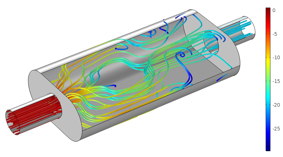 The intensity field depicted using streamlines in an example of an absorptive muffler system (using a porous liner material) at 1300 Hz. The color scale is in dB relative to the inlet intensity.
The intensity field depicted using streamlines in an example of an absorptive muffler system (using a porous liner material) at 1300 Hz. The color scale is in dB relative to the inlet intensity.
The intensity field depicted using streamlines in an example of an absorptive muffler system (using a porous liner material) at 1300 Hz. The color scale is in dB relative to the inlet intensity.
Knowing the intensity (vector field distribution) in a system is useful when analyzing the energy transport and dissipation. The figure above shows the intensity through an absorptive muffler system. The integral of the intensity over a boundary, like the inlet and outlet in the above muffler, gives the total power input/output of the system. Specifically, knowing the combination of incident and reflected waves at a boundary can be used to compute a transmission loss; that is, the ratio between the transmitted power and the incident power. For loudspeaker systems, the integral of the normal intensity over a closed surface defines the radiated power.
The calculation and prediction of absorbed acoustic energy in, for example, human tissue or porous materials also involves the intensity. Simplified semianalytical expressions typically involve knowing the intensity, like the plane wave absorption law  , where
  is the dissipated power density (SI unit: W/m3) and
  is the imaginary part of the wave number.
Boundary Conditions
When solving the governing equations, it is mathematically necessary to close the equations with appropriate boundary conditions. These conditions describe how the acoustic field is generated, how it behaves at boundaries, and how it behaves as it radiates in an infinite domain.
In situations with no mean background flow, the multiphysics nature of acoustics appears at boundaries where the sound field interacts with its surroundings. At the boundary to an elastic structure, the acoustic field will experience the acceleration of the structure, while the structure experiences the pressure load. This is the typical vibroacoustic coupling or acoustic-structure interaction.
Mathematically speaking, two conditions apply at the interface: a kinematic condition stating continuity in displacement (or velocity) and a dynamic condition stating continuity in stress. At the surface of a sound source, like a speaker, sound is not only generated but also impacts the speaker with an added mass and couples back all the way to the electrical source.
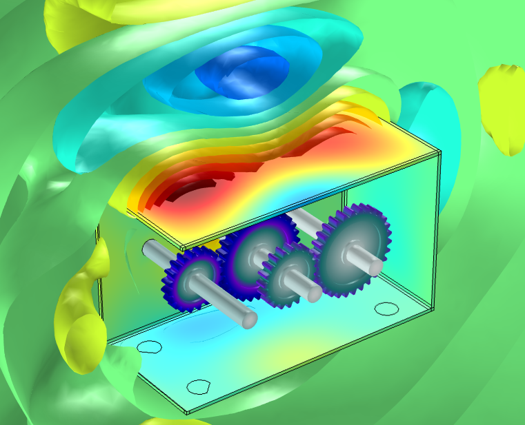 Example of acoustic-structure interaction, where sound is emitted by a gear train assembly inside a box.
Example of acoustic-structure interaction, where sound is emitted by a gear train assembly inside a box.
Example of acoustic-structure interaction, where sound is emitted by a gear train assembly inside a box.
As already discussed, impedance models can be used as boundary conditions to model the behavior of a complex system in a simplified manner; for example, specifying the impedance at the surface of a porous absorber instead of modeling it in detail (Ref. 14 and 15). Impedance conditions are widely used in computational acoustics to reduce the complexity of a model. The impedance models can be seen as engineering relations, as they approximate the true behavior of a complex system but simplify its description. Using an impedance condition can often give a good first approximation to a complex problem.
The behavior of the acoustic waves as they enter or leave a system is described by radiation conditions or port conditions. This class of conditions is especially important in numerical simulations where idealized conditions cannot always be used. At the inlet of a system, like a waveguide, waves should be allowed to enter the guide, while reflected waves should be allowed to exit. This is one example of a radiation or nonreflecting boundary condition (NRBC). At the inlet and outlet of ducts, this type of condition can be implemented as a so-called port condition. In an open system where waves can freely propagate toward infinity, they have to fulfill the Sommerfeld radiation condition, as the distance from sources and scatterers tends to infinity.
In numerical simulations, the proper implementation and formulation of this condition is important in order to avoid spurious numerical reflections that can pollute the solution. A classical example of this type of condition is given by Bayliss, Gunzburger, and Turkel (Ref. 23).
Using a so-called sponge layer to mimic an infinite open problem can be an alternative to a boundary condition. This is a domain where outgoing waves are killed with little or no reflections. One such layer method is the well-known perfectly matched layer (PML). Other formulations also exist for time domain problems where real coordinate stretching is combined with artificial numerical diffusion. In general, these are referred to as absorbing layers.
Equivalent Fluid Models
When acoustic waves propagate in, for example, porous material or a narrow duct, the loss mechanics involved can be complex to describe and model from first principles. In other situations, where a detailed description of the loss mechanism exists, it can be difficult to find analytical or numerical solutions to the problem. In these cases, it can be advantageous to use a so-called equivalent fluid model to describe the loss process in a homogenized way. The typical application is when solving the Helmholtz equation, where the losses are included by defining a complex-valued density  and speed of sound
  (both parameters are typically frequency dependent).
Many equivalent fluid models exist to describe losses in porous materials; for example, the Delany–Bazley–Miki model (Ref. 14, 15, and 24) and the Johnson–Champoux–Allard model (Ref. 14). The idea is to describe the frequency-dependent effective fluid density  and the effective fluid bulk modulus
  of the combined equivalent fluid-solid system (the saturating fluid and porous matrix). The validity of the models are restricted to certain parameter ranges representing the rigid or limp porous matrix approximations. In numerical simulations, an equivalent fluid model is also computationally less demanding than a full poroelastic wave model solving Biot's equations.
When acoustic waves propagate in narrow regions, the losses (viscous and thermal) associated with the acoustic boundary layer need to be taken into account. In most cases, this requires solving the full linear thermoviscous acoustics equations. For narrow slits or waveguides of constant cross sections, homogenized models exist. They are often referred to as low-reduced-frequency models (see the Thermoviscous Acoustics section).
Homogenized equivalent fluid models are also used in underwater acoustics, where losses are defined by an attenuation coefficient  . Values are typically frequency dependent and given in nepers per meter, dB per kilometer, or dB per wavelength (Ref. 12).
Elastic Waves in Solids
When acoustic pressure waves interact with a solid, the fluid’s pressure fluctuations cause a fluid load on the solid domain and the structural acceleration affects the fluid domain as a normal acceleration across the fluid-solid boundary. The propagation of sound in a solid happens through small-amplitude elastic oscillations of the solid's shape and structure.
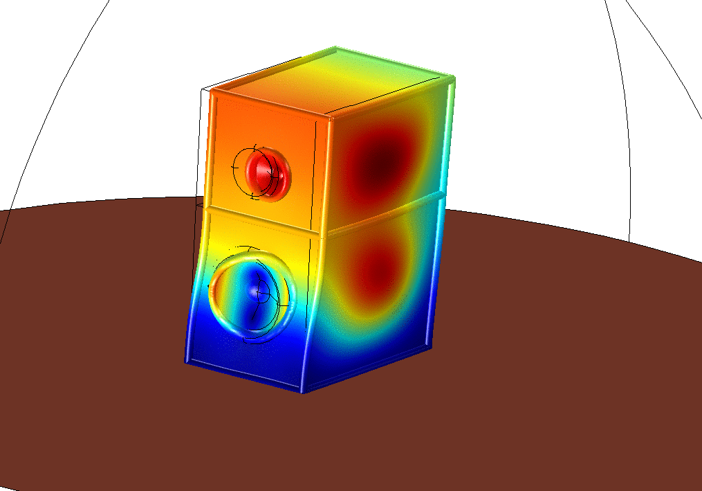
Example of the vibration analysis of a loudspeaker cabinet (the deformation amplitude is exaggerated for visualization). Simulations can be used to identify vibration modes that radiate sound in an unwanted manner from a loudspeaker system.
The equations that govern the propagation of linear elastic waves in solids are derived from the general governing equations of structural mechanics. The equations are linearized and formulated in the limit of small perturbations in the stress and strain. The most general linear relation between the stress and strain tensors in solid materials can be written as

where  is the Cauchy stress tensor, is the strain tensor, and
  is the (fourth-order) elasticity tensor.
This is Hooke's law for a linear elastic material. For small perturbations, the strain tensor (on vector form) is given by

where is the displacement field (SI unit: m).
The elastic wave equation is obtained from Newton's second law (conservation of momentum) and is given by

where is the material density (SI unit: kg/m3) and  and are possible sources.
In the frequency domain, the dependent variable and sources are decomposed into their Fourier components. The resulting Helmholtz-like equation for the elastic waves in a solid is given by
(15)

where is the angular frequency.
Poroelastic Waves
Poroelastic waves describe the combined propagation of pressure waves and elastic waves in porous materials. The pressure waves propagate in the saturating fluid in the pores and the elastic waves propagate in the porous matrix frame. In the limit where the porous matrix frame is almost motionless (rigid), homogenized equivalent fluid models exist to describe the acoustic behavior. The same is true in the limp limit, where the frame follows the movement of the fluid. This description is not generally true for all frequencies or material parameters. Moreover, when the porous material is in contact with a vibrating solid surface, the elastic waves also need to be included. The model that describes the combined propagation solving for both the displacement and the pressure is given by the Biot theory.
 Example of a plane acoustic wave impinging on a sediment layer, described using Biot's theory. The direction of the wave is shown with arrows and the infinite half plane is below the black line. The colors represent the resulting total acoustic field in the air (interference pattern) and inside the porous material. The grayscale represents the total displacement of the porous matrix.
Example of a plane acoustic wave impinging on a sediment layer, described using Biot's theory. The direction of the wave is shown with arrows and the infinite half plane is below the black line. The colors represent the resulting total acoustic field in the air (interference pattern) and inside the porous material. The grayscale represents the total displacement of the porous matrix.
Example of a plane acoustic wave impinging on a sediment layer, described using Biot's theory. The direction of the wave is shown with arrows and the infinite half plane is below the black line. The colors represent the resulting total acoustic field in the air (interference pattern) and inside the porous material. The grayscale represents the total displacement of the porous matrix.
In his seminal work from 1956, Biot extended the classical theory of linear elasticity to porous media saturated with fluids (see Ref. 16–18). In Biot’s theory, the bulk moduli and compressibilities are independent of the wave frequency and can be treated as constant parameters. The porous matrix is described by linear elasticity. Damping is introduced by considering the frequency-dependent losses due to viscosity and thermal conduction of the saturating fluid in the pores. The formulation of the Biot equations that include the thermal effects is sometimes referred to as the Biot–Allard theory (see Ref. 14, 19, and 20). One form of the governing equations is

where  is the fluid density;
  is the average density of the fluid-solid system; and
  is the Biot–Willis coefficient (SI unit: 1), which describes the nature of the fluid frame coupling from rigid
  to limp
  . The Biot–Willis coefficient is assumed constant in space in this formulation.
The complex-valued density and wave number are defined as

where  is the tortuosity (SI unit: 1) or structural form factor (high-frequency limit),
  is the porosity (SI unit: 1),
  is the permeability (SI unit: m2) related to the flow resistivity, and
  is the drained bulk modulus of the matrix (the bulk modulus when in vacuum).
The two frequency-dependent quantities, the viscosity function  and the fluid compressibility
  , include information about the viscous and thermal losses, respectively. The governing equations can be recognized as the elastic waves equation (15) with a diagonal stress source term (defined through the pressure) and the Helmholtz equation (14) with a force source term (defined through the displacement).
Numerical Methods and Computational Acoustics
In order to use the governing equations of acoustics (presented above in the Detailed Derivation of the Governing Equations section) to, for example, predict the behavior of a transducer or the response of a room, they need to be solved numerically in a computational framework. The equations only have a limited number of analytical solutions that are not applicable to realistic geometries, complex boundary conditions, or multiphysics applications. There are many techniques available to solve the governing equations of acoustics, and each has its weaknesses and strengths. Typically, different methods are used for different applications.
The first choice made when solving an acoustic problem is whether to solve the wave equation in the frequency domain or time domain. This is, of course, a generalization, as there are methods that rely on both approaches. For all formulations, the method needs to resolve the waves in both time/frequency and space, taking the frequency content, wavelength, geometry details, possible acoustic boundary layers, and more into account.
The equations can then be solved using one of many methods:
- Finite element method (FEM)
- Integral methods, like the boundary element method (BEM)
- Discontinuous Galerkin (DG) methods
- High-frequency methods, like ray tracing and beam tracing
- Finite difference time domain (FDTD)
- Wave-based methods
- Finite volume methods
- Wave number integration techniques
- Normal modes
- Parabolic equation methods
Note that in the field of aeroacoustics, there is a dedicated discipline called computational aeroacoustics, or CAA, that deals with solving the interaction between flow and acoustics.
Types of Analysis in Acoustics
Pressure Acoustics
In pressure acoustics, only one dependent variable is used to represent the acoustic field: the pressure. The scalar wave equation (13) is solved in the time domain and the Helmholtz equation (14) is solved in the frequency domain. This is, in some sense, classical acoustics.
These equations are adequate to describe acoustics in many situations; for example, scattering and radiation problems, muffler systems, car cabin acoustics, and much more. In their general form, the equations can be used to model problems with nonconstant density and speed of sound, as necessary in underwater acoustics or for multiphysics problems that have a background temperature distribution.
Both equations can be solved with a large variety of boundary conditions. In the frequency domain, equivalent fluid models (homogenization) make it possible to add complex loss effects in porous media and narrow waveguides in a simplified way. Impedance boundary conditions can be used to model the interaction with complex surroundings.
Acoustics and Multiphysics
Acoustic-Structure Interaction
The multiphysics analysis of the interaction of elastic waves in solids and pressure waves in fluids is referred to as acoustic-structure interaction or vibroacoustics. This is a special version of fluid-structure interaction (FSI) valid for acoustics.
Acoustic structure interaction is important in most real-life applications where sound is generated by a vibrating surface or transmitted through structures. Applications include the design and optimization of mufflers, loudspeakers, sound insulation problems, and machine acoustics.
Poroelastic Waves
In porous materials, Biot's equations are solved, accounting for the coupled propagation of elastic waves in the porous matrix and pressure waves in the saturating pore fluid. This includes the damping effect of the pore fluid on the combined wave propagation.
Examples of poroelastic applications range from the propagation of elastic waves in rocks, soils, and sediment to modeling the acoustic attenuation properties of particulate filters, sound absorbers, and porous linings in car cabins.
Piezoacoustics
Piezoacoustics is a multiphysics phenomenon that accounts for the generation and detection of acoustic signals by piezoelectric materials. Piezoelectric transducers are the most prominent application area for piezoacoustics. They are used, for example, in underwater sonar applications.
Acoustic Waves in Pipes
In pipe systems where there is a main guided direction of propagation of the acoustic waves, the mathematical description can be simplified. The effects in the cross section of the pipe can be integrated out, reducing a 3D problem to a set of 1D equations. This highly simplifies the numerical handling of large pipe systems. The effects of the elastic walls of the piping can also be included by modifying the effective compressibility of the fluid.
Electroacoustics
Electroacoustics deals with the generation and detection of acoustics signals by electromechanoacoustic transducers. This includes loudspeakers; headphones; microphones; MEMS transducers; and, in recent years, modeling and designing audio components in mobile devices (to a great extent).
Modeling these devices represents real multiphysics applications where two-way couplings between physics is important. Simulations may include fully detailed models of electromagnetics, structural mechanics, and acoustics solved with, for example, the finite element method or combining FEM with lumped representations using circuit/SPICE diagrams.
Thermoviscous Acoustics
When modeling or studying miniature acoustic devices, like mobile devices, microphones, hearing aids, and perforates, it is essential to include the physical effects described by the thermoviscous acoustic equations in order to predict their correct behavior and response. In particular, the losses associated with the viscous and thermal acoustic boundary layers are important.
It is the thickness of these layers, as compared to the characteristic geometry size, that determines if the device is small in this context. Thermoviscous acoustics also precisely predicts the transition from adiabatic to isothermal behavior in the small gaps that exist in, for example, condenser microphones.
Aeroacoustics
The study of aeroacoustics is concerned with the interaction between a background mean flow and an acoustic field. This includes the generation of sound by flow turbulence or periodic flow structures as well as the influence a flow has on the acoustic field.
Examples of applications include muffler design, where the mean flow can greatly affect the muffler performance; Coriolis flow meters; and, of course, jet engine noise generation and propagation.
There are many formulations of the governing equations solved in aeroacoustics problems. They include acoustic analogy equations, linearized formulations, and solving the full nonlinear flow problem in all of its details. Some examples are:
- Lighthill's acoustic analogy equation
- Linearized Navier–Stokes equation
- Linearized Euler equation
- Linearized potential flow equation
- Acoustic perturbation equations (APE)
- Direct numerical simulation (DNS) of the full compressible flow equations
Geometrical Acoustics
Geometrical acoustics includes methods to solve acoustic problems in the high-frequency limit, where the wavelength is much smaller than the geometrical features. This includes ray tracing methods that assume that sound moves along rays or tubes. The methods are used for modeling room, concert hall, and car cabin acoustics. There are also wide applications in underwater acoustics, outdoor noise propagation, and sound mapping.
Energy Methods
Another class of methods used to solve large-scale acoustics problems are the so-called energy methods. They include statistical energy analysis (SEA) methods, energy finite element methods (EFEM), and other forms of acoustic diffusion equations. The methods do not resolve the acoustic waves, but are limited to the energy transport of acoustic waves and vibrations. The methods are used in complex, coupled systems like cars and houses, as well as for pure indoor room acoustics.
Underwater Acoustics
Underwater acoustics deals with the propagation of sound in the ocean and in other bodies of water. It includes the study of the interaction with the ocean floor (seabed) and sea surface as well as with submerged bodies, like submarines. As sound propagates over long distances in the ocean, effects such as attenuation and the change of speed of sound and density with depth become important. Typical application areas include sonar, seismic exploration, underwater communication, and marine biology.
Nonlinear Acoustics
When the amplitude of the acoustic waves becomes large enough, the linear assumption most often used is no longer valid. As an example, propagating wave troughs and crests will no longer move at the same speed, and signals get distorted. Other effects, like vorticity and very large timescale and size differences, can also give rise to nonlinear phenomena. In order to capture these effects, nonlinear acoustics formulations need to be used or the full compressible flow equations may have to be solved.
Nonlinear effects are often encountered in ultrasound applications, including ultrasound imaging and scanning, where high amplitudes are necessary. Certain imaging techniques actually rely on the nonlinearity and second harmonic generation to enhance resolution. Nonlinear effects due to vorticity generation can be seen in loudspeaker ports as well as in perforates, where they can cause distortion. In microfluidics (acoustofluidics), acoustophoretic effects such as acoustic streaming and radiation forces are caused by accumulated nonlinear contributions that arise from very large timescale differences.
Last modified: Jun 11, 2018
References
D.T. Blackstock, Fundamentals of Physical Acoustics, John Wiley & Sons, 2000.
A.D. Pierce, Acoustics, "An Introduction to Its Physical Principles and Applications," Acoustical Society of America, 1991.
S. Temkin, "Elements of Acoustics," Acoustical Society of America, 2001.
P.M. Morse and K.U. Ingard, Theoretical Acoustics, McGraw Hill (Princeton University Press), 1986.
H. Bruus, Theoretical Microfluidics, Oxford University Press, 2010.
G.K. Batchelor, An Introduction to Fluid Dynamics, Cambridge University Press, 2000.
L.D. Landau and E. M. Lifshitz, Fluid Mechanics, Course of Theoretical Physics, Volume 6, Butterworth-Heinemann, 2003.
B. Lautrup, Physics of Continuous Matter, Exotic and Every Day Phenomena in the Macroscopic World, 2nd ed., CRC Press, 2011.
M.K. Myers, "Transport of energy by disturbances in arbitrary steady flow," J. Fluid Mech. 226, pp. 383–400, 1991.
F.V. Hunt, "Notes on the Exact Equations Governing the Propagation of Sound in Fluids," J. Acoust. Am. 27, pp. 1019–1039, 1955.
C.M. Bender and S.A. Orszag, Advanced Mathematical Methods for Scientists and Engineers: Asymptotic Methods and Perturbation Theory, Springer, 1999.
F.B. Jensen, W.A. Kuperman, M.B. Porter, and H. Schmidt, Computational Ocean Acoustics, Springer, 2011.
H. Kuttruff, Room Acoustics, CRC Press, 2009.
J.F. Allard and N. Atalla, Propagation of Sound in Porous Media, Modeling Sound Absorbing Materials, 2nd Edition, John Wiley & Sons, 2009.
T.J. Cox and P. D’Antonio, Acoustic Absorbers and Diffusers, Taylor and Francis, 2nd ed., 2009.
M.A. Biot, “Theory of Propagation of Elastic Waves in a Fluid-saturated Porous Solid. I. Low-frequency Range,” J. Acoust. Soc. Am., vol. 28, pp. 168–178, 1956.
M.A. Biot, “Theory of Propagation of Elastic Waves in a Fluid-saturated Porous Solid. II. Higher Frequency Range,” J. Acoust. Soc. Am., vol. 28, pp. 179–191, 1956.
M.A. Biot, “Generalized Theory of Acoustic Propagation in Porous Dissipative Media,” J. Acoust. Soc. Am., vol. 34, pp. 1254–1264, 1962.
J.F. Atalla, R. Panneton, and P. Debergue, "A mixed displacement-pressure formulation for poroelastic materials," J. Acoust. Soc. Am., vol. 104, pp. 1444–1452, 1998.
J.F. Atalla, M.A. Hamdi, and R. Panneton, "Enhanced weak integral formulation for the mixed (u-p) poroelastic equations," J. Acoust. Soc. Am. vol. 109, pp. 3065–3068, 2001.
J.W.S. Rayleigh, The Theory of Sound: Introduction by R.B. Lindsay, Dover Publications, 1945.
R.B. Lindsay, "The Story of Acoustics," J. Acoust. Soc. Am., vol. 39, pp. 629–644, 1966.
A. Bayliss, M. Gunzburger, and E. Turkel, “Boundary Conditions for the Numerical Solution of Elliptic Equations in Exterior Regions,” SIAM J. Appl. Math., vol. 42, no. 2, pp. 430–451, 1982.
Y. Miki, “Acoustical properties of porous materials - modifications of Delany-Bazley models,” J. Acoust. Soc. Jpn (E), vol. 11, no. 1, 1990.
M.F. Hamilton and D.T. Blackstock (edited by), Nonlinear Acoustics, Acoustical Society of America, 2008.
P. Barkholt Muller and H. Bruus, "Numerical study of thermoviscous effects in ultrasound-induced acoustic streaming in microchannels," Phys. Rev. E 90, 043016 1–12, 2014.