
Introduction to Structural Mechanics
What Is Structural Mechanics?
Structural mechanics, or solid mechanics, is a field of applied mechanics in which you compute deformations, stresses, and strains in solid materials. Often, the purpose is to determine the strength of a structure, such as a bridge, in order to prevent damage or accidents. Other common goals of structural mechanics analyses include determining the flexibility of a structure and computing dynamic properties, such as natural frequencies and responses to time-dependent loads.
The study of solid mechanics closely relates to material sciences, since one of the fundamentals is to have appropriate models for the mechanical behavior of the material being used. Different types of solid materials require vastly different mathematical descriptions. Some examples are metals, rubbers, soils, concrete, and biological tissues.
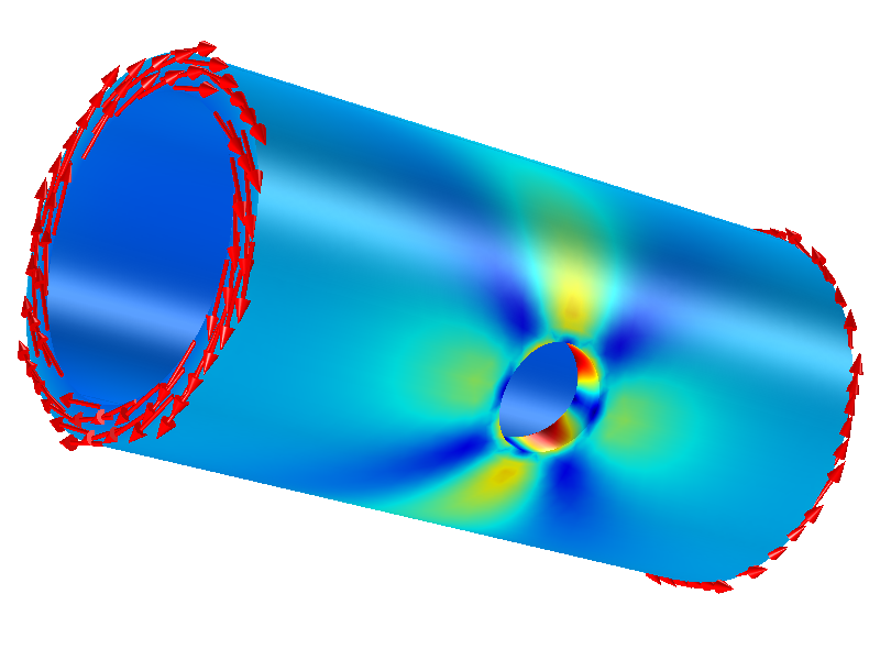 Stresses at a hole in a twisted tube. Geometrical transitions often cause local stress concentrations.
Stresses at a hole in a twisted tube. Geometrical transitions often cause local stress concentrations.
Stresses at a hole in a twisted tube. Geometrical transitions often cause local stress concentrations.
Three Fundamental Relations in Structural Mechanics
Within mechanics, structures may be statically determinate or statically indeterminate. In the first case, all forces in a system can be computed purely by equilibrium considerations. In real life, static indeterminacy is common, at least when it comes to computing the internal stress distribution in a component. In a statically indeterminate system, the deformations must be taken into account in order to compute the forces.
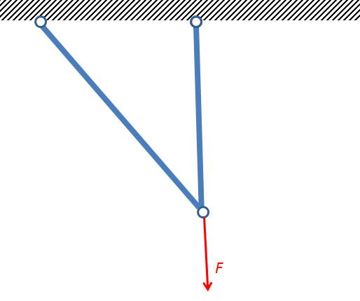 A statically determinate structure. The forces in the two bars can be determined from the balance of the horizontal and vertical forces of the joint where the force is applied.
A statically determinate structure. The forces in the two bars can be determined from the balance of the horizontal and vertical forces of the joint where the force is applied.
A statically determinate structure. The forces in the two bars can be determined from the balance of the horizontal and vertical forces of the joint where the force is applied.
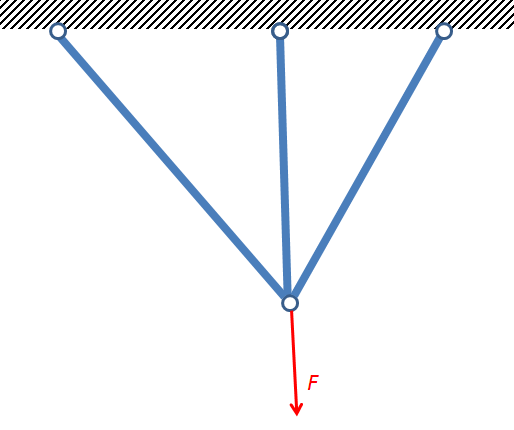 A statically indeterminate structure. The forces in three bars cannot be determined by only two force balance equations at the joint. The force distribution is influenced by the stiffness of each bar.
A statically indeterminate structure. The forces in three bars cannot be determined by only two force balance equations at the joint. The force distribution is influenced by the stiffness of each bar.
A statically indeterminate structure. The forces in three bars cannot be determined by only two force balance equations at the joint. The force distribution is influenced by the stiffness of each bar.
Due to the static indeterminacy, almost all structural mechanics analyses rely on the same three types of equations, which express equilibrium, compatibility, and constitutive relations. These equations can, however, come in different guises, depending on whether the analysis is at a continuum level or a large-scale structural level.
Stress and Equilibrium Equations
The equilibrium equations are based on Newton's second law, stating that the sum of all forces acting on a body (including any inertial forces) sum up to zero, so that all parts of any structure must be in equilibrium. If you make a virtual cut through a material somewhere, there must be forces in the cut that are in balance with the external loads. These internal forces are called stresses.
 The external forces on a bar are balanced by the internal stresses.
The external forces on a bar are balanced by the internal stresses.
The external forces on a bar are balanced by the internal stresses.
In three dimensions, the stresses in the material are represented by the stress tensor, which can be written as

An element in the stress tensor represents a force component on a unit area in the material. One index is the direction of the force component and the other index is the orientation of the normal to the surface on which the force acts. From moment equilibrium considerations, the stress tensor is symmetric and contains six independent values.
In terms of the stresses, Newton's second law can be formulated as

where  is a force per unit volume,
  is the mass density, and
  is the displacement vector.
Strain and Compatibility Equations
Compatibility relations are requirements on the deformations. For example, in a framework, the ends of all members joined at a point must move the same distance and in the same direction.
Inside the material, the local deformations are characterized by the strain that represents a relative deformation. For a simple elongation of a bar, the engineering strain,  , is a ratio of the displacement,
  , and the original length,
  .
.
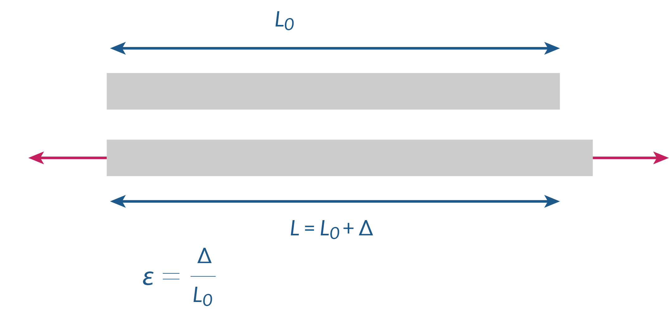 Definition of the engineering strain for pure extension.
Definition of the engineering strain for pure extension.
Definition of the engineering strain for pure extension.
In a general 3D setting, the strain is also represented by a symmetric tensor,

where the individual elements are defined as derivatives of the displacements,

The individual components of the strain tensor cannot have arbitrary spatial distributions, since they are derived from a displacement field. This provides the compatibility conditions for a continuum. These compatibility conditions, either on the structure level or the continuum level, are basically geometric relations. Just as the equilibrium relations, these conditions are fundamental and do not contain any assumptions.
Constitutive Relations
A constitutive relation, that is, a material model, forms the bridge from force to deformation or from stress to strain. As opposed to the two previous sets of equations, constitutive relations cannot be derived from first principles, but are purely empirical. The laws of thermodynamics, symmetry conditions, and similar arguments can at best provide some limitations on the allowed mathematical structure of the material models.
Mathematically, material models relate stresses to strains. In a few cases, for elastic materials, this relation is unique. Often, the relation also includes time derivatives (as in viscoelasticity) or a memory of previous strains (as in plasticity).
For each material, it is necessary to perform measurements and then fit these measurements to a suitable mathematical model.
Linear Elastic Materials
The most fundamental material model is linear elasticity in which stresses are proportional to strains. On the structural level, linear elasticity means that, for example, the deflection of a beam is proportional to the load applied to it. In practice, this material model is often sufficient.
An isotropic linear elastic material can be characterized by two independent material constants, often chosen as the modulus of elasticity (Young's modulus), E, and Poisson's ratio,  .
.
Consider a bar with cross section A and length L, subjected to an axial force F:
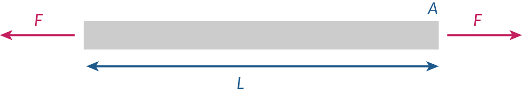 An axially loaded bar.
An axially loaded bar.
An axially loaded bar.
The axial stress is the ratio between the force and the cross-section area,

If the measured elongation is Δ, then the axial strain is

The modulus of elasticity gives the relation between the axial stress and axial strain:

The proportionality between stress and strain, or between force and displacement, is called Hooke's law. Combining the equations above gives the stiffness relation for the bar as

Usually, the bar in tension not only extends, but also shrinks in the transverse direction. The relation between the strain in the transverse directions and the strain in the axial direction is given by Poisson's ratio:

The 3D generalization of Hooke's law can be written as

where D is a symmetric 6×6 matrix. In the most general anisotropic case, the matrix contains 21 independent constants. For the isotropic case, it is only a function of E and :

Other Material Models
There are many families of material models for structural mechanics applications. Within each family, there are several possible models. In the table below, you can find a few examples.
| Material Model Family | Examples | Common Material Models |
|---|---|---|
| Linear elastic | Many materials at small strains, e.g.: metals |
• Hooke's law • Isotropic and anisotropic |
| Elastoplastic, volume preserving | Metals at larger strains |
• Tresca • von Mises |
| Elastoplastic, mean stress dependent | Soils |
• Mohr-Coulomb • Drucker-Prager |
| Creep | Metals at elevated temperatures |
• Norton • Garofalo |
| Hyperelastic | Rubbers, biological tissues |
• Mooney-Rivlin • Ogden |
| Viscoelastic | Plastics |
• Maxwell • Kelvin • Standard linear solid |
Navier's Equations
For an isotropic linear elastic solid, it is possible to formulate a system of three partial differential equations (PDEs) for the displacement vector , which summarizes all aspects of the problem. This will give Navier's equations, which can be written as

where  and
and  are two independent material constants, called the Lamé parameters.
In terms of E and , Navier's equation can also be written as

For more general cases, it is not possible to formulate the solid mechanics equations explicitly in terms of the displacements. In these instances, a coupled set of equilibrium, constitutive, and compatibility equations must be solved.
Boundary Conditions
To complete the formulation of the solid mechanics problem, appropriate boundary conditions must be applied.
Prescribed Displacements
Usually, the displacements are known on some parts of the boundaries of the body. A building, for example, rests on the ground. If the known displacements are not sufficient to suppress all possible rigid body motions, it is not possible to fully determine the displacement field. When the external loads are known, it may still be possible to compute the stresses, since the absolute displacements will not be of interest. Numerical solutions will, however, typically require a sufficient set of prescribed displacements.
Mathematically, prescribed displacements provide a Dirichlet condition.
Forces
In the majority of solid mechanics analyses, external forces are part of the problem formulation.
Forces may be volumetric, like gravity or centrifugal forces. Such loads are part of the governing PDE itself, not boundary conditions.
There are, however, also loads acting on the boundaries such as the internal pressure in a pipe or the force from the snow on a roof. The latter are true Neumann boundary conditions. In some cases, the orientation of the load changes with the deformation. This is called a follower load. Such loads give rise to a nonlinear problem, since the load causes a deformation that then changes the load.
Springs
Elastic foundations can be considered as a mixture of the two previous types. Here, the force acting on the structure is a function of the displacement. They are often proportional. Mathematically, this is a Robin boundary condition. As an example, the soil under a building cannot always be considered as giving a zero displacement, so its flexibility must be accounted for in this way. Elastic supports are an alternative to prescribed displacements when it comes to suppressing rigid body motions.
Stationary and Dynamic Problems
The general Newton's second law contains the inertial forces from acceleration. In many cases, the loads vary slowly and the dynamic terms can be ignored. This assumption is very common in practical engineering. Such a formulation is called static, stationary, or quasistatic.
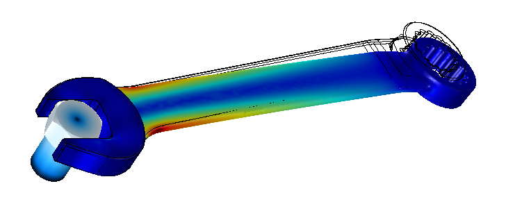 The tightening of a bolt can usually be considered by a static analysis, since vibrations in the wrench are not of interest.
The tightening of a bolt can usually be considered by a static analysis, since vibrations in the wrench are not of interest.
The tightening of a bolt can usually be considered by a static analysis, since vibrations in the wrench are not of interest.
Eigenfrequencies
A structure always has some mass. The combination of inertia with elasticity, through Newton's second law, gives rise to differential equations with second-order time derivatives. This can be seen in Navier's equations, for example, which are discussed above. Such equations typically possess wave-type solutions. Using the appropriate boundary conditions and assuming a harmonic solution, the resulting equation system presents an eigenvalue problem. Solving the eigenvalue problem gives a set of eigenvalues, called eigenfrequencies or natural frequencies.
From the physical point of view, it means that an elastic structure will have the tendency to vibrate at certain distinct frequencies. For each eigenfrequency, the corresponding deformation pattern is called eigenmode.
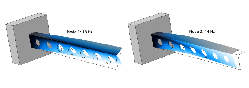 The first two eigenmodes of a cantilever beam.
The first two eigenmodes of a cantilever beam.
The first two eigenmodes of a cantilever beam.
Determining a structure's eigenfrequencies is central to almost all dynamic analyses, since it indicates the frequencies at which resonances can be expected. By knowing the eigenfrequencies, it is possible to see if the time scale of a certain load is such that it can cause dynamic amplification.
Dynamic Loading
When loads have a temporal variation with a time scale comparable to the period time for some of the natural frequencies of a structure, it is necessary to take the dynamic response into account. Dynamic loads can be divided into deterministic and random loads. In the case of deterministic loads, the histories of all loads affecting the structure are completely known. This is often the case in machine components. Random-type loads, on the other hand, will not have a predictable time history, except possibly in an average sense. Wind loads and earthquake loads belong to this category.
Time-Dependent Loads
The most general description of a deterministic load is by the full time history. In order to compute the displacements and stresses, the governing differential equations must be solved together with an appropriate set of initial conditions. Often, this is done numerically with some type of time-stepping algorithm.
Harmonic Loads
In practice, it is very common for loads to have a harmonic variation. This is often the case in rotating machines. If the structure has a linear behavior, then the response is also harmonic as soon as any start-up transients have died out. Such problems can be solved efficiently in the frequency domain. If the frequency of a harmonic load is close to a natural frequency of the structure, then there is a significant amplification of the response when compared to a stationary solution. At resonance, that is when the loading frequency exactly matches a natural frequency, the vibration amplitude can become very large. The displacements are only limited by the damping in the structure, which is often low.
For harmonic loading, it is common to study the frequency response. This means that you analyze the response for many loading frequencies and the results are presented as a function of the frequency.
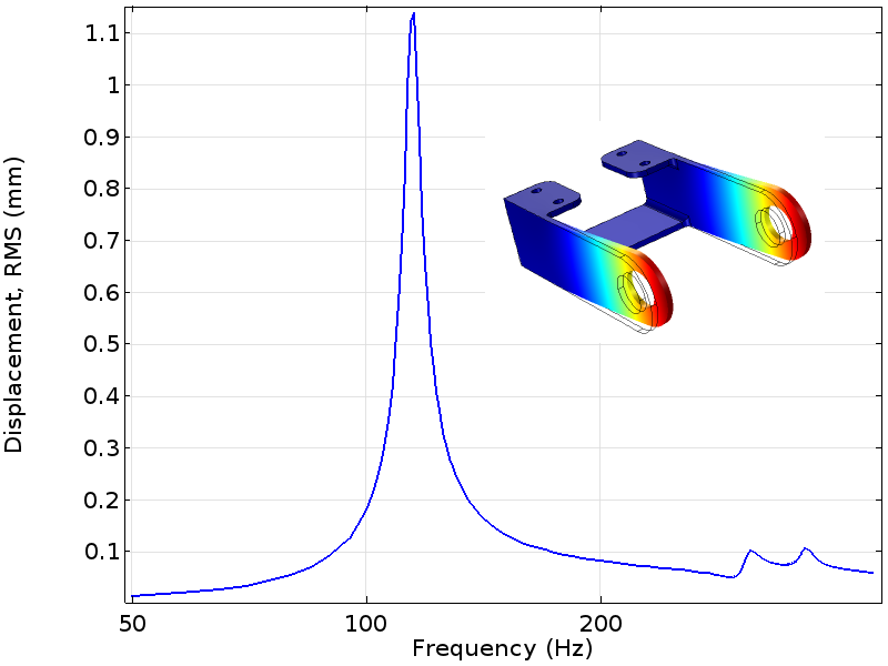 A frequency response analysis of a bracket. The natural frequency at 115 Hz causes a distinct resonance peak, whereas the two eigenmodes with frequencies around 300 Hz are not excited to the same extent.
A frequency response analysis of a bracket. The natural frequency at 115 Hz causes a distinct resonance peak, whereas the two eigenmodes with frequencies around 300 Hz are not excited to the same extent.
A frequency response analysis of a bracket. The natural frequency at 115 Hz causes a distinct resonance peak, whereas the two eigenmodes with frequencies around 300 Hz are not excited to the same extent.
If the problem is nonlinear, as when mechanical contact is involved, the response will no longer be harmonic even if the loads are harmonic. Such problems must, in most cases, be solved as general time-dependent problems.
Random Loads
As an example of a random load, consider the wind load on a tall building. The average wind speed varies along the tower, but there are also wind gusts, which have random strength and duration. Furthermore, the gusts are not always synchronous when studying different locations on the structure. If a number of measurements are available, then it is in theory possible to perform a time-dependent analysis for each measurement. However, this does not cover any future events, since they will not be exactly identical to those already measured.
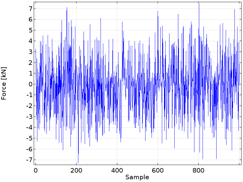 A measured random load history.
A measured random load history.
A measured random load history.
For random load cases, the load is best described by its statistical properties. This description is usually given in the form of power spectral density (PSD). The response to such a load in terms of displacements or stresses is then also described in statistical terms.
Approximations for Slender Geometries
Long before the introduction of numerical simulation, engineers realized that it was possible to analyze some types of structures using simplified theories. Beam theory applies to long slender bodies, while plate and shell theory is useful for thin sheets that are flat or curved. In these cases, assumptions about the stress and strain variation in the cross-sectional directions makes it possible to perform important approximations to the general equations. Before the availability of finite element software, very few fully 3D problems could be solved. Analytical solutions for many plate, shell, and beam configurations have, however, been available for a long time and have been used extensively in engineering calculations.
Beam Theory
In beam theory, a structure is treated with a 1D formulation for the deformation of the center line of the beam. The perpendicular directions are only represented by cross-section properties such as area and moments of inertia. In a beam analysis, the distribution of forces and moments along the beam is often the primary result. The determination of stresses from these quantities is a trivial operation due to the underlying assumptions.
For beams with a constant cross section, which is most common, many analytical solutions exist and can be found in handbooks.
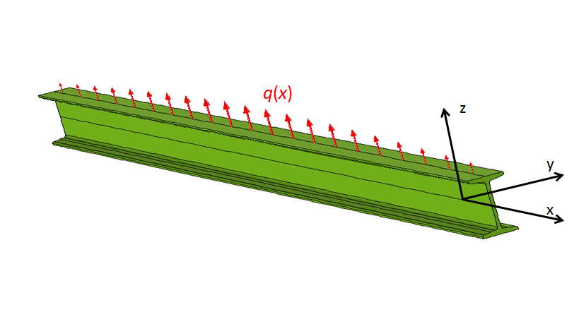 A beam with distributed load q(x).
A beam with distributed load q(x).
A beam with distributed load q(x).
The governing differential equation for bending of a slender beam in the xz-plane is

where w is the deflection, E is the modulus of elasticity,  is the area moment of inertia around the y-axis, and q is the load per unit length in the z-direction.
When the cross section is constant, the equation can be directly integrated to

where the last term represents the primitive function of the load distribution, integrated four times.
For a dynamic case, the equation of motion is

where is the mass density and A is the cross-section area.
The theory for slender beams is often referred to as Euler-Bernoulli theory. If the height of the beam is not small compared to the beam length, such theory is no longer sufficient because it ignores the shear deformations. Timoshenko beam theory can instead be used as a proper extension for thicker beams.
Plates
Plate theory can be applied to thin flat plates where the load is acting in the perpendicular direction. The formulation is 2D, so that the thickness direction is only present through the value of the thickness. The plate carries the load by bending action, just as a beam does. Plate theory is often used in civil engineering, for example, when analyzing floors or bridge decks.
As in the case of beams, different versions of plate theory exist for thin and thick plates. The thin plate theory is often referred to as Kirchhoff theory, whereas the thick plate theory, which includes transverse shear deformations, is known as Mindlin theory. For a thin plate with a constant thickness h and an isotropic elastic material, the partial differential equation for bending is

where the bending stiffness D is given by

The deflection is denoted by w and q is the distributed load per unit area.
It is also possible to include the effect of an in-plane load in the theory. A tensile in-plane load acts stiffening on the plate, whereas a compressive in-plane load acts softening and may even cause the plate to buckle.
Shells
A shell can be considered as a plate with a midsurface that is curved in space. Due to the curvature, there is a strong coupling between in-plane and bending action. Analytical or tabulated results for shells are not available to the same extent as for plates and beams and are mostly limited to geometries exhibiting rotational symmetry.
Due to their curvature, shells are very efficient load-carrying structures. Eggs, for example, are amazingly strong. Pressure vessels can often be analyzed by shell theory.
Membranes
For very thin structures, like rubber balloons or pieces of cloth, you can apply membrane theory. In membrane theory, the material does not resist a transverse loading by bending action, but by membrane action.
Contact Problems
In many mechanical devices, objects come into contact with each other. This is the case, for example, during mounting processes, in roller bearings, and in impact situations. Such problems are strongly nonlinear, since the contact area depends on the force pressing the two objects together. Typically, the maximum contact pressure varies as the square root or cube root of the applied force, since the force is distributed over a larger area as the indentation increases.
Analytical solutions to contact problems are available for only a few cases. The famous Hertzian contact solutions describe the stress field and contact areas for some combinations of elastic objects, such as two spheres or a cylinder and a plane.
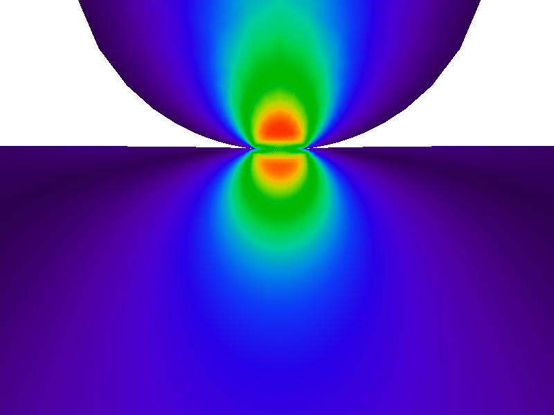 Equivalent stress at the contact between a cylinder and an elastic half plane.
Equivalent stress at the contact between a cylinder and an elastic half plane.
Equivalent stress at the contact between a cylinder and an elastic half plane.
In many cases, you must take into account the friction between two objects in the analysis. Friction modeling is difficult, not only from a mathematical point of view, but also since the coefficient of friction between two surfaces can depend on many different parameters, including their cleanliness.
In practice, contact problems are almost always solved with numerical techniques, like the finite element method.
Failure Mechanisms
The purpose of a structural mechanics analysis is often to verify the integrity of a structure, so it is necessary to have failure criteria. For real-life designs, the allowed loads are reduced by a safety factor to allow for uncertainties in material data, manufacturing tolerances, and analysis assumptions. The size of the safety factor depends on several factors, where the severity of the consequence of a failure is one of the most important factors.
Think about it: It is better to have a higher risk of failure in a gardening tool than in a nuclear plant.
Static Failure
Static failure occurs if the loads to which a structure is subjected cause a stress that at a certain moment exceeds the strength of the material.
The ultimate strength of a material is the stress at which it breaks, which is usually measured in a uniaxial test. The ultimate strength, however, is not a true material property. To some extent, it also depends on the geometry of the test specimen.
Materials are often classified as brittle or ductile. A brittle material, like glass, is more or less elastic until it reaches its ultimate strength at a rather small strain. A ductile material, like a mild steel, is elastic up to the yield stress. Then, it experiences a large amount of plastic deformation before it finally breaks. With a ductile material, the deformations can become so large that a component is no longer fit for service, while still not being fully ruptured.
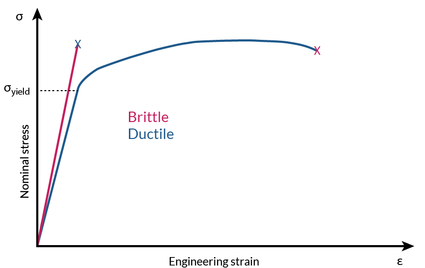 Tensile tests for brittle and ductile materials.
Tensile tests for brittle and ductile materials.
Tensile tests for brittle and ductile materials.
Fatigue
Material fatigue occurs when a crack forms in a structure after many repeated load cycles, where the stress in each cycle can be far below the ultimate stress. Fatigue is considered to be the most common cause of structural failures in service.
The number of cycles required to cause fatigue damage can be anywhere between a few cycles up to several million cycles, depending on the stress amplitude in each load cycle. Once a crack in a structure is initiated, it continues to grow with each load cycle. Finally, the damaged component is no longer able to sustain the peak load. The fatigue life is influenced not only by the amplitude of the stress cycle, but also the mean stress. A tensile stress state is more damaging than a compressive one.
The fatigue properties of a certain material are strongly influenced by factors like surface roughness and service environment.
Fracture Mechanics
When a crack is present in a structure, you can no longer use the standard criteria for maximum allowable stresses, since the strain at a sharp crack tip tends to infinity. The behavior of cracks are studied within the field of fracture mechanics. In linear elastic fracture mechanics (LEFM), the severity of a crack is characterized by stress intensity factors (KI, KII, KIII) for normal, in-plane shear, and out-of-plane shear, respectively.
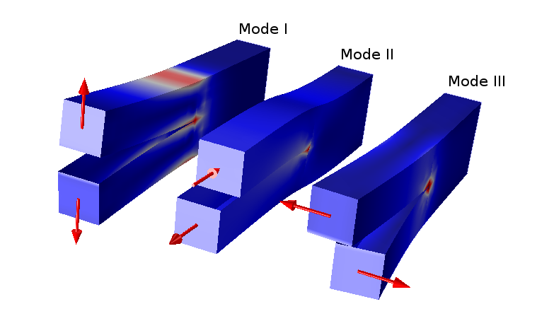 The three modes in fracture mechanics analysis.
The three modes in fracture mechanics analysis.
The three modes in fracture mechanics analysis.
If the load is cyclic, but it is small enough not to cause an immediate failure, then the crack growth per cycle can be predicted by LEFM, for example, with Paris' law.
Often, there is significant plastic deformation around the crack tip. In that case, methods for elastoplastic fracture mechanics (EPFM) must be used. This includes J-integrals and energy release rate methods.
Buckling
Some types of structures, typically slender structures predominantly under compression, can fail due to a phenomenon known as buckling. At a certain load, the structure becomes unstable and the deformation suddenly increases, often to the level of a total collapse. You can illustrate this phenomenon by pressing a plastic ruler between your hands. Nothing happens at first, until the ruler suddenly assumes a curved shape.
 The buckling of a metal measuring tape under compression.
The buckling of a metal measuring tape under compression.
The buckling of a metal measuring tape under compression.
Mathematically, buckling occurs when a bifurcation point — where there are two or more possible solutions — has been reached. This problem is inherently geometrically nonlinear. It is only when the equilibrium equations are formulated in a deformed state that the secondary, possibly unstable, branch can be detected.
Types of Multiphysics Analyses in Structural Mechanics
The deformation of solid objects often interacts strongly with other physical phenomena. In some cases, such as when a loudspeaker membrane emits sound waves, this is intentional. In other cases, like when a sun kink is formed on a railroad by the thermal expansion of the rail steel, deformation is highly undesirable.
Here are some cases in which other physical effects interact with structural mechanics phenomena.
Thermal-Structure Interaction
The most common type of thermal-structure interaction is thermal expansion. The volume of most materials increases with temperature. Solid materials characteristically increase in length with 10–100 ppm/K. This change can cause large stresses in a constrained component. Also, when mixing materials with different coefficients of thermal expansion, temperature changes cause stresses because of the mismatch in thermal expansion.
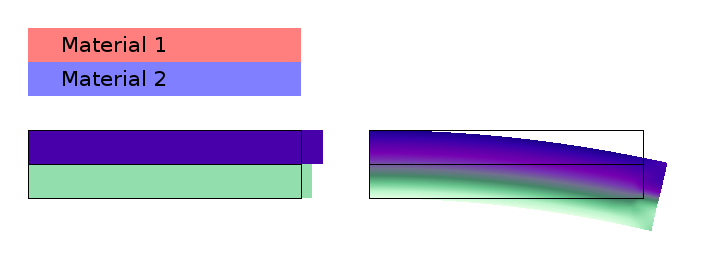 Strains in two materials with different coefficients of thermal expansion, heated to a common elevated temperature. Left: The two materials are sliding on top of each other and do not interact. Right: The materials are joined at the common boundary, so that a bimetallic spring is formed. The bending is caused by the mismatch in extension. As a side effect, there is a compressive stress in the upper layer and a tensile stress in the lower layer.
Strains in two materials with different coefficients of thermal expansion, heated to a common elevated temperature. Left: The two materials are sliding on top of each other and do not interact. Right: The materials are joined at the common boundary, so that a bimetallic spring is formed. The bending is caused by the mismatch in extension. As a side effect, there is a compressive stress in the upper layer and a tensile stress in the lower layer.
Strains in two materials with different coefficients of thermal expansion, heated to a common elevated temperature. Left: The two materials are sliding on top of each other and do not interact. Right: The materials are joined at the common boundary, so that a bimetallic spring is formed. The bending is caused by the mismatch in extension. As a side effect, there is a compressive stress in the upper layer and a tensile stress in the lower layer.
There are also cases where deformations in a solid can cause heating. For example, in metal forming, large inelastic strains are induced. The energy is then dissipated as heat and it is possible for the temperature to increase of the order of 100 K in a short time.
Even in elastic situations, strains are accompanied by small but reversible changes in temperature. However, the order of magnitude is of the order of mK, so it can be ignored in most cases. On some size and frequency scales, most commonly the high-frequency vibrations in MEMS structures, this heating is responsible for an appreciable amount of damping. This is called thermoelastic damping.
Larger changes in temperature also change the material data. At elevated temperatures, both the stiffness and strength of the material decrease significantly. New phenomena, like creep deformations, may also become important at higher temperatures.
Hygroscopic swelling
Some materials, such as wood and many engineering polymers, can absorb significant amounts of moisture. This will cause swelling as well as changes in mass density. The effect of the swelling is similar to that of thermal expansion. For some materials, the volume changes can, however, be orders of magnitude larger than what is the case for thermal expansion.
Typically, the moisture content is controlled by a diffusion process. The diffusivity can be influenced by the structural stresses, but in most cases, this effect can be ignored.
One field of application where hygroscopic swelling is important is in the analysis of electronics packaging. The epoxies used for this purpose have a significant ability to absorb humidity from the surroundings, which can cause shape changes and stresses.
Fluid-Structure Interaction
Fluids and structures can interact in several ways. The pressure and viscous forces in a fluid cause a load on the boundary of the structure. For example, the pressure in a pipe is usually the main source of loading.
If a structure is relatively flexible, the load from the fluid also causes a deformation that can change the flow pattern. Such bidirectional couplings can explain phenomena as diverse as snoring and wing flutter in aircrafts.
Acoustic-Structure Interaction
Sound waves, or pressure fluctuations in gases and fluids, often interact with vibrations in surrounding solid objects. The pressure in an acoustic medium acts as a load on the solid material, while the acceleration of the solid is transmitted as an acceleration at the boundary of the deformable medium, thus causing pressure waves. Both of these effects can be intentional, as in loudspeakers or microphones. But it is also common for the coupling to be a source of undesirable noise transmission, as when sound is transmitted through the walls in a building.
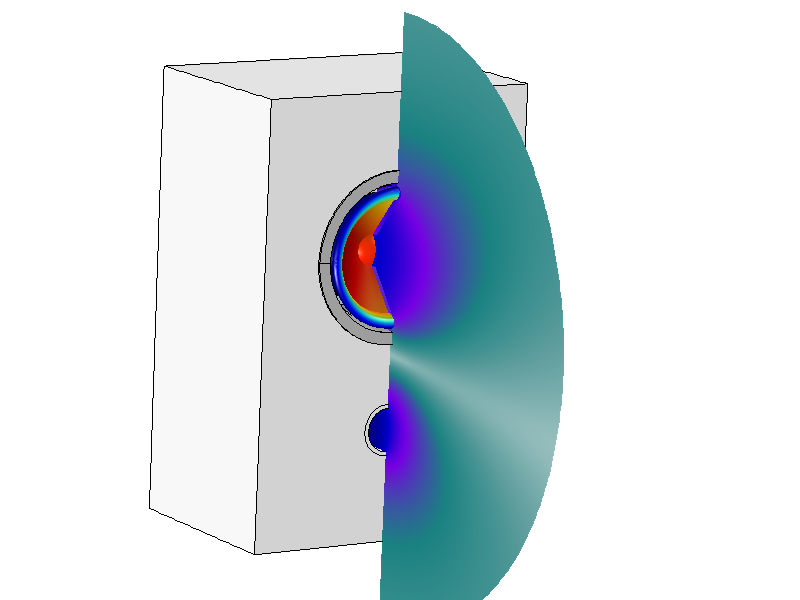 The displacement of a speaker membrane and the acoustic pressure level in front of the loudspeaker.
The displacement of a speaker membrane and the acoustic pressure level in front of the loudspeaker.
The displacement of a speaker membrane and the acoustic pressure level in front of the loudspeaker.
Piezoelectricity
Piezoelectricity is the bidirectional coupling between an electric field and strain in some dielectric materials. Usually, the relation is linear. This phenomenon can be utilized in many ways, for example, for controlling mechanical deformation by an electric potential or for energy harvesting in which mechanical deformations are converted to electric power. Piezoelectricity is also used for triggering the spark in some cigarette lighters, for example.
Piezoresistivity
In a piezoresistive material, the electric resistivity of a material depends on the strain. This effect, which is observed in metals and semiconductors, is useful for various types of sensors. In particular, piezoresistivity is often used in strain gauges, which are the most common devices for measuring small strains.
Electrostriction
Electrostriction is an interaction between an electric field and strain in a structure, and it occurs in all dielectric materials. As opposed to piezoelectricity, the strains are proportional to the square of the electric polarization.
Magnetostriction
Magnetostriction is a similar phenomenon to electrostriction, but in this case, the coupling is between a magnetic field and mechanical strain. There are a few specially engineered materials for which this coupling is very strong and these materials are used in efficient sensors and transducers. Magnetostriction also causes the humming sound that is sometimes emitted by electrical equipment like transformers.
Published: April 19, 2018Last modified: April 19, 2018