support@comsol.com
Results and Visualization Updates
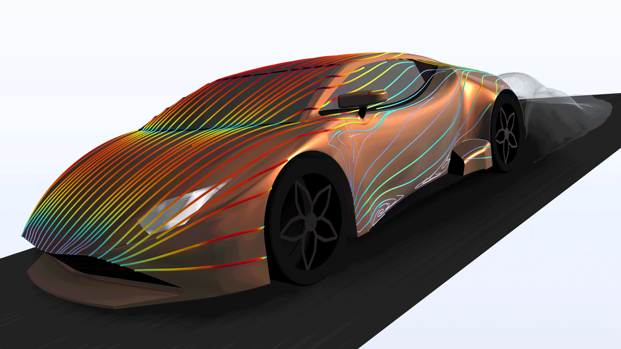
COMSOL Multiphysics® version 6.2 provides improved functionality for creating streamline plots, new contour and isosurface series plots, and the ability to enhance 3D and depth perception with floor shadows. Read about these updates and more below.Improved Streamline Plots
The functionality for creating streamline plots has been improved significantly. Streamline plots can now be created on curved surfaces using the existing Streamline Surface plot type. In addition, the algorithm for creating uniform and magnitude-controlled streamlines provides improved handling and efficiency as well as updates for enhanced visualization.
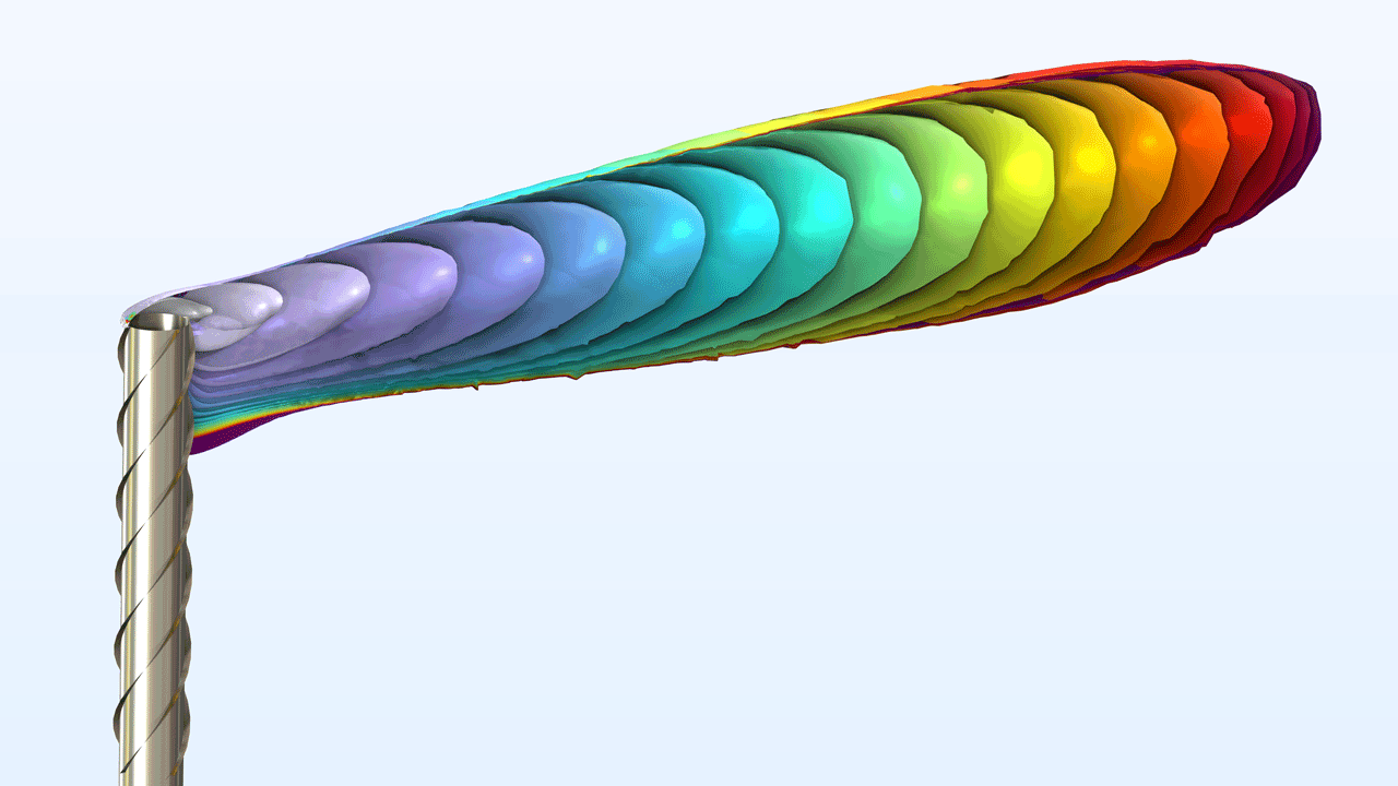
Contour Series and Isosurface Series Plots
The new Contour Series and Isosurface Series plots are used for visualizing field level progression over time. For example, the Isosurface Series plot effectively displays the dispersion of a pollutant plume over time by visualizing specific concentration values as isosurfaces versus time.
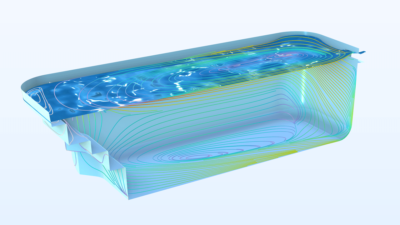
Floor Shadows
To further increase 3D and depth perception, a new visual effect, Floor Shadows, has been introduced. This effect is easily accessible from the Graphics window toolbar. In the feature's settings, you can select the light sources that produce the shadow and define their positions. You can also modify the position of the floor plane as well as the sharpness and darkness of the shadow.
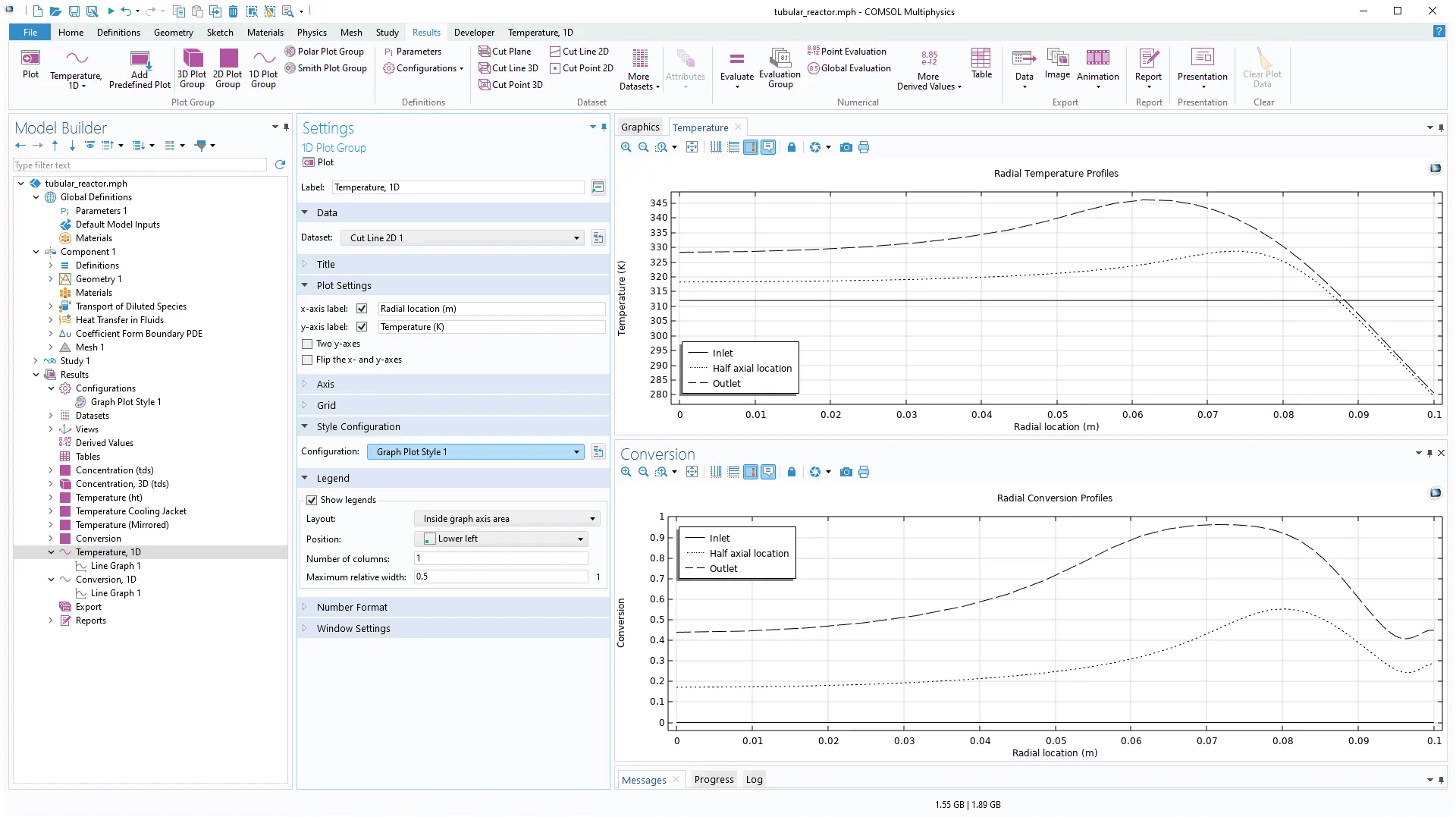
Configurations
In the Model Builder, it is now possible to add configurations by right-clicking the Results node and choosing Configurations from the resulting context menu. There are three options: Graph Plot Style, Multiselect Solution, or Single-Select Solution. These configurations offer centralized control over plot groups, enabling uniformity of style and dataset values across multiple plot groups without the need to adjust the settings for each group individually. Each of these three options controls an entire selection of plot groups in the model tree and can be used to simultaneously update its respective plot groups. The Multiselect Solution and Single-Select Solution configurations also offer control over derived values and evaluation groups.
With the Single-Select Solution and Multiselect Solution options, it is possible to set solution parameters from a common configuration. For 2D and 3D plot groups, the Single-Select Solution option can be used, for example, to generate several plots with the same time data. The Multiselect Solution option can be used for 1D plots to show multiple solutions over a parametric sweep or multiple time steps. With the Graph Plot Style option, line width and line styles can be set for several plot groups of graph plots (xy-plots) in order to create same-style plots.
The configuration options save time, increase the quality of presentations and reports, and make it easier and much quicker to plot the right data and control plots in simulation apps.
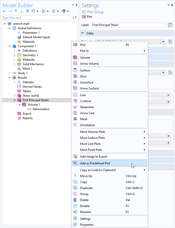
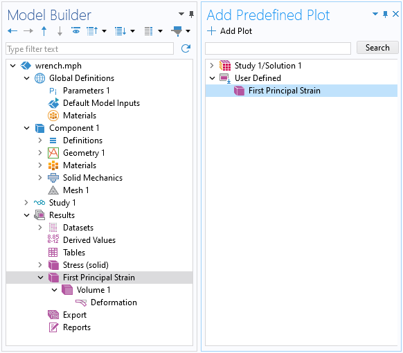
User-Defined Predefined Plots
It is now possible to add your favorite plots to the Add Predefined Plot window for reuse in other models. To do so, select Add as Predefined Plot in the context menu of plot groups, evaluation groups, or derived values nodes. The predefined plots that are added appear in the User Defined category in the Add Predefined Plot window. These saved predefined plots will remain available for any sessions run on the same computer.
Interactive Result Extraction in Graph Plots
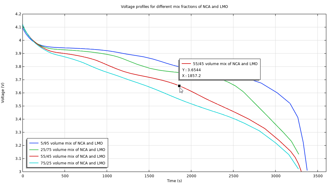
For graph plots (xy-plots), interactive result extraction is now available with the Enable Tooltip button in the Graphics window toolbar. With this feature enabled, tooltips with values and plot data information will appear when you hover the mouse cursor over points on the graph. This makes it easier to extract precise quantitative information from plots.
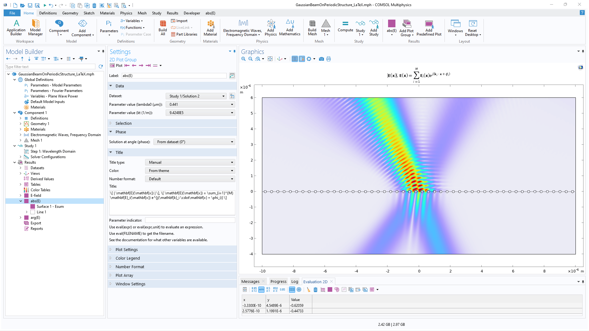
Mathematical Expressions in Titles
In this version, plot titles have been improved to support new lines, truncation, and LaTeX mathematical expressions. Two types of escape sequences are supported that will enable math modes, where one uses a LaTeX display math mode and the other uses a LaTeX inline math mode.
- Display math mode: Place [ ] around the LaTeX mathematical expression in the title text field. This mode uses more vertical space for the math expression, but it does not add a new line like the mode does for normal LaTeX.
- Inline math mode: Place \$ \$ around the LaTeX mathematical expression in the title text field. This mode is meant to be inlined in the text (in normal LaTeX) and has a more compact presentation.
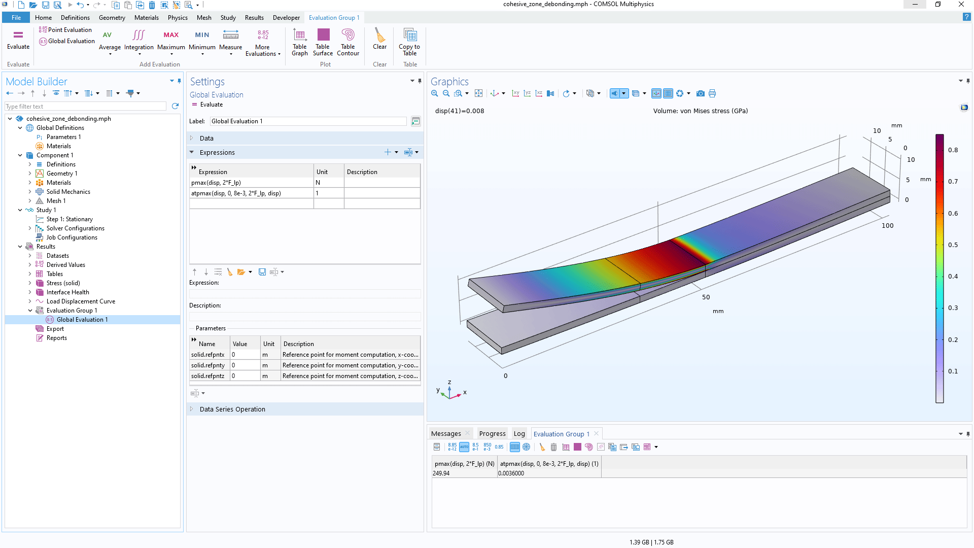
Operators for Evaluation over a Parametric Sweep
There are new built-in operators (atpmax, atpmin, pmax, and pmin) for the integration, summation, and evaluation of the maximum and minimum values of a parameter sweep solution. These operators enhance the functionality for evaluating the results of parameter sweep studies.
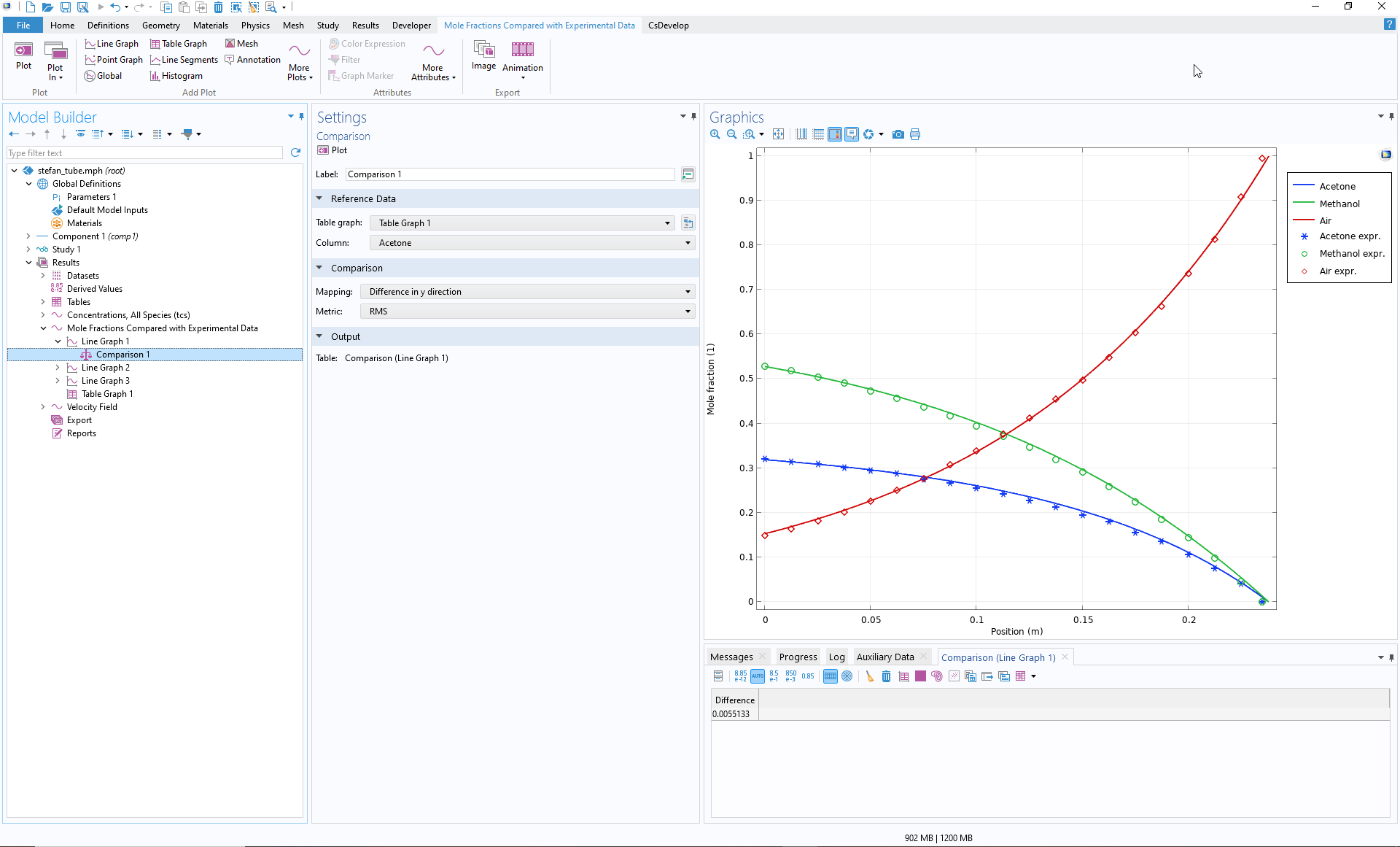
Comparing Graph Plots and Reference Data
The new Comparison plot subnode is used for comparing two plots:
- A graph plot that shows the value of an expression in a simulation
- A table graph plot that contains reference data (typically experimental data)
There are several metrics (such as RMS) available for comparing the two sets of plot data. The result of the comparison, a scalar value, is shown in a table located below the Graphics window.