AC/DC Module Updates
For users of the AC/DC Module, COMSOL Multiphysics® version 5.3a offers a new physics interface called Magnetic Fields, No Currents, Boundary Elements, postprocessing updates to the previously released Electrostatics, Boundary Elements interface, a new material model for modeling soft permanent magnets, and a new Surface Magnetic Current Density boundary condition. Check out all of the AC/DC Module updates in more detail below.
New and Updated Boundary Element Interfaces
A new physics interface has been developed based on the boundary element method (BEM): the Magnetic Fields, No Currents, Boundary Elements interface. It solves for the scalar magnetic potential and can be used as a standalone interface to model permanent magnets with linear, constant, and homogeneous properties. The interface also provides multiphysics coupling features for combining finite element method (FEM) and BEM modeling of more complex scenarios when used together with the finite-element-based Magnetic Fields, No Currents and Magnetic Fields interfaces. For example, hybrid FEM-BEM models can be used to model nonlinear anisotropic magnetic materials based on an FEM formulation with a surrounding domain that utilizes the new Magnetic Fields, No Currents, Boundary Elements interface.
Introduced with COMSOL Multiphysics® version 5.3, the Electrostatics, Boundary Elements interface has been enhanced with support for electrostatic force calculations and new postprocessing variables on boundaries. Additionally, postprocessing and visualization of boundary-element-based fields has been improved with automatic smoothing near boundaries.
 A submarine with its magnetic signature 1 km below it. The box and submarine have been magnified by a factor of 20 in the plot. In this model, the boundary element method is used to model the open space outside the box, whereas the finite element method is used to model the submarine and its immediate vicinity.
Updated Interface for Rotating Machinery
The Rotating Machinery, Magnetic interface in the AC/DC Module now uses an updated version of the moving mesh functionality. The moving mesh settings are now shared between physics interfaces, avoiding duplication of settings. This facilitates multiphysics modeling in moving domains with greater ease as compared to previous versions. Among other benefits, this makes it much easier to combine electromagnetics with fluid flow in rotating machinery.
Material Model for Soft Permanent Magnets
A new material model for modeling soft permanent magnets has been added to the Magnetic Fields; Magnetic Fields, No Currents; and Rotating Machinery, Magnetic interfaces. A generic example material Demagnetizable Nonlinear Permanent Magnet with the approximate properties of AlNiCo 5 has been added to the AC/DC material database to serve as a template for user-defined materials supporting the new material model. Two important permanent magnet materials are AlNiCo (soft magnet) and NdBFe (hard magnet). AlNiCo magnets have an advantage over NdBFe magnets at elevated operating temperatures since the Curie temperature for AlNiCo magnets is in the range 700–860°C as opposed to 310–400°C for NdBFe magnets. For this reason, AlNiCo is sometimes used in permanent magnet (PM) motors where temperatures may be too high for NdBFe magnets. A key design consideration for such motors is that the magnetic flux density in the magnets must never drop below the "knee" of the magnetization curve as that would result in irreversible demagnetization and loss of performance.
 Soft permanent magnet example: When the flux path of the soft permanent magnet (cylinder) is closed by the iron core (gray), the soft magnetic material stays in the safe region above the knee of its magnetization curve. When moved into free air, it goes below the knee and will not return along the original curve, but instead follow the dotted red line. It will suffer from permanent demagnetization.
When moved into free air, the soft permanent magnet loses so much of its initial magnetization that the change becomes irreversible.
Magnetic Scalar Potential Discontinuity
When building models using the scalar magnetic potential formulation in the Magnetic Fields, No Currents interface, you can now introduce edge current loops with the Magnetic Scalar Potential Discontinuity feature. This feature is available when enabling Advanced Physics Options and may result in models that are more computationally lean and efficient, as compared to using the more general vector potential formulation.
Toroid inductor model with the new Magnetic Scalar Potential Discontinuity feature applied on the gray circular boundaries, equivalent to imposing a line current of 1[kA] along the associated circular edges.
Surface Magnetic Current Density
A surface magnetic current density can now be specified as a 3D vector field embedded in a surface. With the new Surface Magnetic Current Density boundary condition, added to the Magnetic Fields interface, the magnetic current density is projected onto a boundary surface, neglecting its normal component. This allows you to specify a surface magnetic current density at both exterior and interior boundaries of your model. This new boundary condition has been included for special modeling situations, such as the modeling of electric dipoles.
Lamination Modeling Example in the Time Domain
The Rotating Machinery 3D tutorial model has been updated to provide an example of rotor lamination. The rotating cylinder in the model is simulated with and without insulating boundary conditions in the Rotating Machinery, Magnetic interface and the results are compared. When the rotor is laminated, the results show that the eddy current losses are significantly reduced.
 Rotating machinery example where the cylinder rotates around its axis, generating eddy currents from the magnetic field produced by a permanent magnet. The current density is calculated for two situations: without an insulating layer (top image, left legend) and with an insulating layer (bottom image, right legend).
Application Library path:
ACDC_Module/
Magnetic Force Verification Models
Two new tutorial models have been added to the Application Library that calculate the magnetic force and torque, respectively. They are part of a planned series of tutorials using the Magnetic Fields, No Currents and Magnetic Fields, No Currents, Boundary Elements interfaces. Both models compare BEM and FEM to analytical models. The models are meant to serve as an introduction to the boundary element method for magnetostatics.
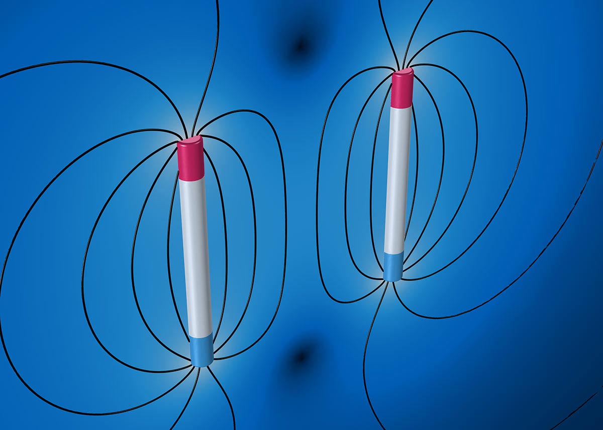
Two parallel magnetized rods of one meter length, placed one meter apart. The remanent flux density inside the rods is chosen such that the analytical model predicts a repelling force between the two rods of exactly one Newton.
Application Library paths:
ACDC_Module/Verification_Examples/force_calculation_02_magnetic_force_bem
ACDC_Module/Verification_Examples/force_calculation_03_magnetic_torque_bem
Updated Tutorial Model: Lumped Loudspeaker Driver Using Lumped Mechanical System
This is a model of a moving-coil loudspeaker where a lumped parameter analogy represents the behavior of the electrical and mechanical speaker components. The Thiele-Small parameters (small-signal parameters) serve as input to the lumped model. In this model, the mechanical speaker components such as moving mass, suspension compliance, and suspension mechanical losses are modeled using the Lumped Mechanical System interface.
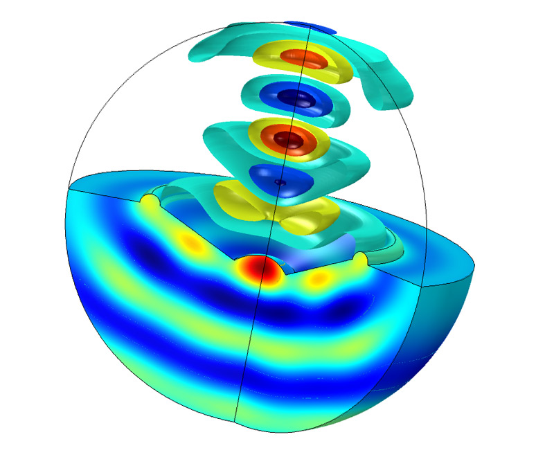 Pressure field plotted as isosurfaces (above the speaker cone) and as a surface plot (below the speaker cone).
Application Library path:
Acoustics_Module/Electroacoustic_Transducers/lumped_loudspeaker_driver_mechanical