Mixer Module Updates
For users of the Mixer Module, COMSOL Multiphysics® version 5.3a brings all turbulence models to rotating machinery, mixture models, and bubbly flow, as well as a revamped modeling workflow for rotating machinery interfaces with moving mesh. Browse these and more Mixer Module updates below.
All Turbulence Models Now Available for Rotating Machinery
The new version of the CFD Module contains ready-made formulations for all of the turbulence models when used in tandem with rotating machinery. This makes it simpler to model turbulent flow with rotating machinery for any turbulence model that previously had to be defined manually, in a rotating frame.
 Model of a centrifugal pump modeled with the new turbulence model and rotating machinery combination.
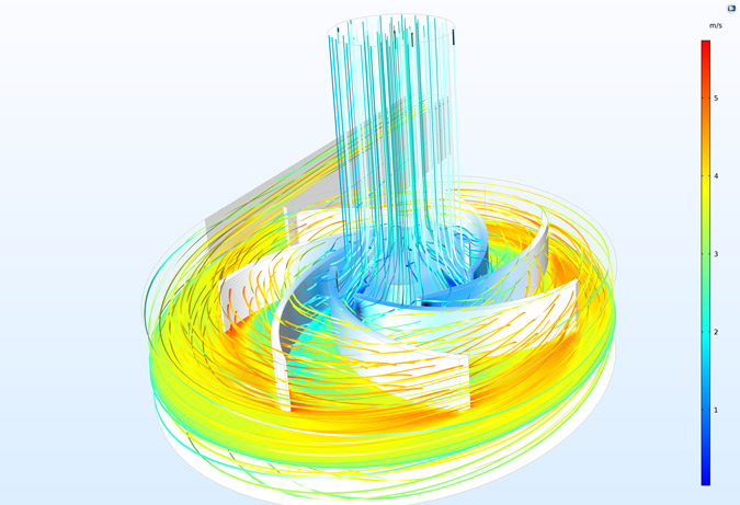
All Turbulence Models Now Available for the Mixture Model and Bubbly Flow Interfaces
The Bubbly Flow and Mixture Model interfaces now include all turbulence models as well as automatic wall treatment, except the inherently wall-law-based k-ε and realizable k-ε formulations. Additionally, interior wall boundary conditions are available, thus making it possible to treat impellers, rotors, baffles, fins, etc. without having to mesh thin walls.
Benchmark model of turbulent bubbly flow, also making use of bubble-induced turbulence. The animation shows the volume fraction of bubbles with a view from below.
Revamped Rotating Machinery Interfaces with Moving Mesh
The Rotating Machinery, Fluid Flow interfaces have been improved by separating the Rotating Domain node from the fluid flow physics. When adding one of these interfaces, the single-phase flow interface is added as well as a Rotating Domain node under Definitions > Moving Mesh. With this separation, you can now combine any fluid flow interface with rotating machinery. Even with this increased flexibility, it is just as easy to define fluid flow in rotating machinery and the separate moving mesh as with previous versions of COMSOL Multiphysics®. The moving mesh controls the spatial frame in a model and may apply to all physics interfaces in a model where the domains are rotating. As an example, this simplifies the combination of fluid flow with chemical species transport in mixers and stirred reactors.
The tutorial model of a gently mixed liquid solution utilizes the new rotating machinery interface for laminar flow. The rotating machinery interface is also available for all turbulence models for more vigorously stirred mixers and tank reactors.
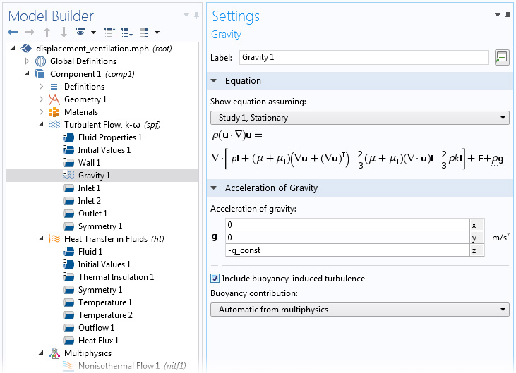
Buoyancy-Induced Turbulence
Buoyancy introduces a volume force in the bulk of a fluid that may naturally cause instabilities. Eventually, these instabilities in the flow become chaotic, leading to the onset of turbulence. The Gravity feature, used for modeling buoyancy in the CFD Module, now includes the option of accounting for buoyancy-induced turbulence by selecting the corresponding check box. This contribution to the turbulent flow can then be defined either automatically from the Nonisothermal Flow multiphysics coupling or from a user-defined turbulent Schmidt number.
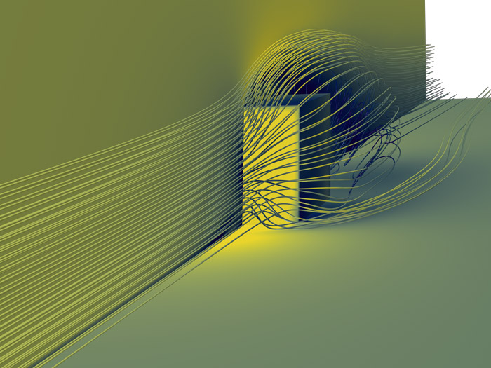
Inlet Boundary Condition for Fully Developed Turbulent Flow
The Inlet boundary condition for fully developed turbulent flow gives the velocity profile and the turbulence variable values at an inlet cross section, assuming that the inlet channel upstream is of a certain length and that the flow is fully developed. In previous versions of the COMSOL® software, a decent estimate of the cross section velocity profile would have required modeling a very long inlet section of the channel. The new boundary condition gives a very accurate inlet profile without the need for extra geometry and therefore reduces the computational resources.
 The inlet from a nozzle with star-shaped cross section is modeled using the fully developed turbulent flow inlet condition.
New Realizable k-ε Turbulence Model Interface
The new Turbulent Flow, Realizable k-ε interface adds a popular RANS turbulence model to your arsenal of turbulence models. Most turbulence models include realizability constraints to ensure nonnegativity of turbulent normal stresses, Schwarz's inequality between any fluctuating quantities, and to limit the production of turbulence. However, the new realizable k-ε turbulence model applies realizability by allowing the coefficients in the turbulence transport equations to vary with respect to the mean flow deformation rate as well as k and ε. This results in a smoother, more physical approach to the limiting states.
 Turbulent flow hitting a cube at a straight angle to one of the faces. The realizable k-ε turbulence model prevents the turbulent energy component in the strain direction from assuming negative values due to rapid mean strain.
New Fluid-Structure Interaction Interface That Supports All Turbulence Models
A new Fluid-Structure Interaction multiphysics coupling has replaced the interface used in previous versions of the COMSOL® software. The new coupling matches the modern style, with a number of single-physics interfaces and multiphysics nodes to couple them together. With this approach, all functionality in the constituent physics interfaces is available for fluid-structure interaction (FSI) modeling. On the structural side, many additional boundary conditions and material models are now available for FSI analysis; for example, rigid domain, piezoelectric, and nonlinear elastic material models. On the fluid side, all turbulence models are now available as well as a number of new boundary conditions. After adding a Fluid-Structure Interaction interface from the Model Wizard, you will get a Solid Mechanics interface, a Laminar Flow interface, a Fluid-Structure Interaction multiphysics coupling node, and a Moving Mesh node in the Definitions section. All fluid-structure interaction models in the Application Libraries have been updated to include this new coupling functionality.
 Pressure (color table) and deformation (exaggerated by a factor of 50 at the surface) of a sports car wing subjected to turbulent flow (streamlines) of 200 km/h (125 mph) in a test bench. The model is defined using one-way fluid-structure interaction in the new physics interface.
Substantially Improved Performance and Stability for Time-Dependent Problems
The solver strategy for time-dependent problems has been modified, resulting in a smoother and more robust solution process that is up to 50% faster without losing any accuracy.
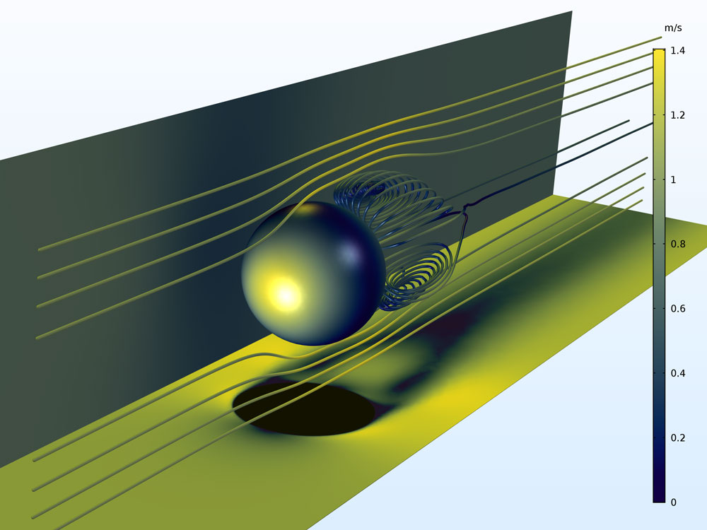
Time-dependent model of the flow around a sphere creating a Karman vortex street downstream, solved more quickly in COMSOL Multiphysics® version 5.3a.